Applies To

Use the Find and Replace features in Excel to search for something in your workbook, such as a particular number or text string. You can either locate the search item for reference, or you can replace it with something else. You can include wildcard characters such as question marks, tildes, and asterisks, or numbers in your search terms. You can search by rows and columns, search within comments or values, and search within worksheets or entire workbooks.

Tip: You can also use formulas to replace text. To learn more, check out the SUBSTITUTE function or REPLACE, REPLACEB functions.

PausedWindowsmacOSWeb

Find

To find something, press Ctrl+F, or go to Home > Editing > Find & Select > Find.

Note: In the following example, we’ve selected Options >> to show the entire Find dialog box. By default, it displays with Options hidden.

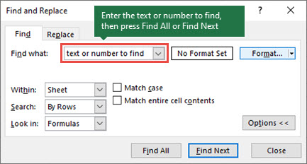
1. In the Find what box, type the text or numbers you want to find, or select the arrow in the Find what box, and then select a recent search item from the list.Tips: 
   • You can use wildcard characters — question mark (?), asterisk (*), tilde (~) — in your search criteria.
   • Use the question mark (?) to find any single character — for example, s?t finds “sat” and “set”.
   • Use the asterisk (*) to find any number of characters — for example, s*d finds “sad” and “started”.
   • Use the tilde (~) followed by ?, *, or ~ to find question marks, asterisks, or other tilde characters  — for example, fy91~? finds “fy91?”.
2. Select Find All or Find Next to run your search.Tip: When you Select Find All, every occurrence of the criteria you’re searching for is listed, and selecting a specific occurrence in the list selects its cell. You can sort the results of a Find All search by selecting a column heading.
3. Select Options>> to further define your search if needed:
   • Within: To search for data in a worksheet or in an entire workbook, select Sheet or Workbook.
   • Search: You can choose to search either By Rows (default), or By Columns.
   • Look in: To search for data with specific details, in the box, select Formulas, Values, Notes, or Comments.Note:   Formulas, Values, Notes and Comments are available only on the Find tab; only Formulas are available on the Replace tab.
   • Match case – Check this if you want to search for case-sensitive data.
   • Match entire cell contents – Check this if you want to search for cells that contain only the characters that you typed in the Find what box.
4. If you want to search for text or numbers with specific formatting, select Format, and then make your selections in the Find Format dialog box.Tip: If you want to find cells that just match a specific format, you can delete any criteria in the Find what box, and then select a specific cell format as an example. Select the arrow next to Format, select Choose Format From Cell, and then select the cell that has the formatting that you want to search for.

Replace

To replace text or numbers, press Ctrl+H, or go to Home > Editing > Find & Select > Replace.

Note: In the following example, we’ve selected Options >> to show the entire Find dialog box. By default, it displays with Options hidden.

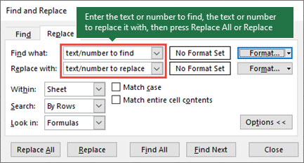
1. In the Find what box, type the text or numbers you want to find, or select the arrow in the Find what box, and then select a recent search item from the list.Tips: 
   • You can use wildcard characters — question mark (?), asterisk (*), tilde (~) — in your search criteria.
   • Use the question mark (?) to find any single character — for example, s?t finds “sat” and “set”.
   • Use the asterisk (*) to find any number of characters — for example, s*d finds “sad” and “started”.
   • Use the tilde (~) followed by ?, *, or ~ to find question marks, asterisks, or other tilde characters — for example, fy91~? finds “fy91?”.
2. In the Replace with box, enter the text or numbers you want to use to replace the search text.
3. Select Replace All or Replace.Tip: When you select Replace All, every occurrence of the criteria that you’re searching for is replaced, while Replace updates one occurrence at a time.
4. Select Options>> to further define your search if needed:
   • Within: To search for data in a worksheet or in an entire workbook, select Sheet or Workbook.
   • Search: You can choose to search either By Rows (default), or By Columns.
   • Look in: To search for data with specific details, in the box, select Formulas, Values, Notes, or Comments.Note:   Formulas, Values, Notes and Comments are available only on the Find tab; only Formulas are available on the Replace tab.
   • Match case – Check this if you want to search for case-sensitive data.
   • Match entire cell contents – Check this if you want to search for cells that contain only the characters that you typed in the Find what box.
5. If you want to search for text or numbers with specific formatting, select Format, and then make your selections in the Find Format dialog box.Tip: If you want to find cells that just match a specific format, you can delete any criteria in the Find what box, and then select a specific cell format as an example. Select the arrow next to Format, select Choose Format From Cell, and then select the cell that has the formatting that you want to search for.

REPLACE function

Applies To

This article describes the formula syntax and usage of the REPLACE function in Microsoft Excel. 

Description

REPLACE replaces part of a text string, based on the number of characters you specify, with a different text string.

Syntax

REPLACE(old_text, start_num, num_chars, new_text)

The REPLACE function syntax has the following arguments:

• Old_text    Required. Text in which you want to replace some characters.
• Start_num    Required. The position of the character in old_text that you want to replace with new_text.
• Num_chars    Required. The number of characters in old_text that you want REPLACE to replace with new_text.
• New_text    Required. The text that will replace characters in old_text.

Example

Copy the example data in the following table, and paste it in cell A1 of a new Excel worksheet. For formulas to show results, select them, press F2, and then press Enter. If you need to, you can adjust the column widths to see all the data.

Data
abcdefghijk
2009
123456
Formula	Description (Result)	Result
=REPLACE(A2,6,5,”*”)	Replaces five characters in abcdefghijk with a single * character, starting with the sixth character (f).	abcde*k
=REPLACE(A3,3,2,”10″)	Replaces the last two digits (09) of 2009 with 10.	2010
=REPLACE(A4,1,3,”@”)	Replaces the first three characters of 123456 with a single @ character.	@456

Important: 

• The REPLACEB function is deprecated.
• In workbooks set to Compatibility Version 2, REPLACE has improved behavior with Surrogate Pairs, counting them as one character instead of two. Variation Selectors (commonly used with emojis) will still be counted as separate characters. Read more here: The Unicode standard