Applies To

A PivotTable is a powerful tool to calculate, summarize, and analyze data that lets you see comparisons, patterns, and trends in your data. PivotTables work a little bit differently depending on what platform you are using to run Excel.

If you have the right license requirements, you can ask Copilot to help you create a PivotTable.

Create a PivotTable in Excel for Windows

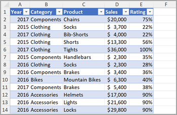
1. Select the cells you want to create a PivotTable from.Note:  Your data should be organized in columns with a single header row. See the Data format tips and tricks section for more details.
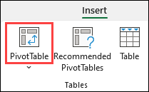
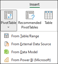
2. Select Insert > PivotTable.
3. This creates a PivotTable based on an existing table or range.
   Note: Selecting Add this data to the Data Model adds the table or range being used for this PivotTable into the workbook’s Data Model. Learn more.
4. Choose where you want the PivotTable report to be placed. Select New Worksheet to place the PivotTable in a new worksheet or Existing Worksheet and select where you want the new PivotTable to appear.
5. Select OK.

PivotTables from other sources

By clicking the down arrow on the button, you can select from other possible sources for your PivotTable. In addition to using an existing table or range, there are three other sources you can select from to populate your PivotTable.

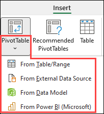
Note: Depending on your organization’s IT settings you might see your organization’s name included in the list. For example, “From Power BI (Microsoft).”

Get from External Data Source

Get from Data Model

Use this option if your workbook contains a Data Model, and you want to create a PivotTable from multiple tables, enhance the PivotTable with custom measures, or are working with very large datasets.

Get from Power BI

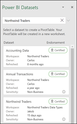
Use this option if your organization uses Power BI and you want to discover and connect to endorsed cloud datasets you have access to.

Building out your PivotTable

1. To add a field to your PivotTable, select the field name checkbox in the PivotTables Fields pane.Note: Selected fields are added to their default areas: non-numeric fields are added to Rows, date and time hierarchies are added to Columns, and numeric fields are added to Values.
2. To move a field from one area to another, drag the field to the target area.

Refreshing PivotTables

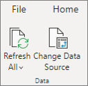
If you add new data to your PivotTable data source, any PivotTables that were built on that data source need to be refreshed. To refresh just one PivotTable, you can right-click anywhere in the PivotTable range, and then select Refresh. If you have multiple PivotTables, first select any cell in any PivotTable, then on the ribbon go to PivotTable Analyze > select the arrow under the Refresh button, and then select Refresh All.

Working with PivotTable Values

Summarize Values By

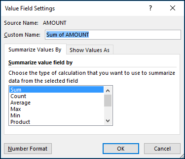
By default, PivotTable fields placed in the Values area are displayed as a SUM. If Excel interprets your data as text, the data is displayed as a COUNT. This is why it’s so important to make sure you don’t mix data types for value fields. You can change the default calculation by first selecting the arrow to the right of the field name, and then select the Value Field Settings option.

Next, change the calculation in the Summarize Values By section. Note that when you change the calculation method, Excel automatically appends it in the Custom Name section, like “Sum of FieldName”, but you can change it. If you select Number Format, you can change the number format for the entire field.

Tip: Since changing the calculation in the Summarize Values By section changes the PivotTable field name, it’s best not to rename your PivotTable fields until you’re finished setting up your PivotTable. One trick is to use Find & Replace (Ctrl+H) >Find what > “Sum of“, and then Replace with > leave blank to replace everything at once instead of manually retyping.

Show Values As

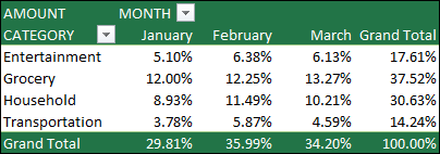
Instead of using a calculation to summarize the data, you can also display it as a percentage of a field. In the following example, we changed our household expense amounts to display as a % of Grand Total instead of the sum of the values.

Once you’ve opened the Value Field Setting dialog box, you can make your selections from the Show Values As tab.

Display a value as both a calculation and percentage.

Simply drag the item into the Values section twice, and then set the Summarize Values By and Show Values As options for each one.

Data format tips and tricks

• Use clean, tabular data for best results.
• Organize your data in columns, not rows.
• Make sure all columns have headers, with a single row of unique, non-blank labels for each column. Avoid double rows of headers or merged cells.
  
  
• Format your data as an Excel table (select anywhere in your data, and then select Insert > Table from the ribbon).
• If you have complicated or nested data, use Power Query to transform it (for example, to unpivot your data) so it’s organized in columns with a single header row.

Filter data in a PivotTable

Applies To

PivotTables are great for creating in-depth detail summaries from large datasets. WindowsWebmacOS

Paused

Filter data in a PivotTable with a slicer

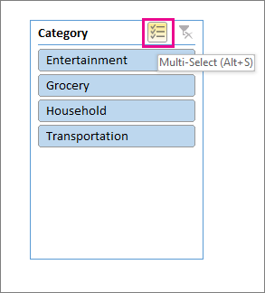
You can insert one or more slicers for a quick and effective way to filter your data. Slicers have buttons you can click to filter the data, and they stay visible with your data, so you always know what fields are shown or hidden in the filtered PivotTable.

1. Select any cell within the PivotTable, then on the Pivot Table Analyze tab, choose   Insert Slicer.
2. Choose the fields you want to create slicers for, and select OK.
3. Excel will place one slicer for each selection you made onto the worksheet, but it’s up to you to arrange and size them however is best for you.
4. Select the slicer buttons to choose the items you want to show in the PivotTable.

Filter data manually

Manual filters use AutoFilter. They work in conjunction with slicers, so you can use a slicer to create a high-level filter, then use AutoFilter to dive deeper.

1. To display AutoFilter, select the  Filter drop-down arrow, which varies depending on the report layout.
   
   Compact Layout   The Value field is in the Rows areaThe Value field is in the Columns areaOutline/Tabular Layout   
   
   
   
   Displays the Values field name in the top left corner
2. To filter by creating a conditional expression, select Label Filters, and then create a label filter.
3. To filter by values, select Values Filters and then create a values filter.
4. To filter by specific row labels (in Compact Layout) or column labels (in Outline or Tabular Layout), uncheck Select All, and then select the check boxes next to the items you want to show. You can also filter by entering text in the Search box.
5. Select OK.

Tip: You can also add filters to the PivotTable’s Filter field. This also gives you the ability to create individual PivotTable worksheets for each item in the Filter field. For more information, see Use the Field List to arrange fields in a PivotTable.

Show the top or bottom 10 items

You can also apply filters to show the top or bottom 10 values or data that meets the certain conditions.

1. To display AutoFilter, select the  Filter drop-down arrow, which varies depending on the report layout.
   
   Compact Layout   The Value field is in the Rows areaThe Value field is in the Columns areaOutline/Tabular Layout   
   
   
   
   Displays the Values field name in the top left corner
2. Select Values Filters > Top 10.
3. In the first box, select Top or Bottom.
4. In the second box, enter a number.
5. In the third box, do the following:
   • To filter by number of items, pick Items.
   • To filter by percentage, pick Percentage.
   • To filter by sum, pick Sum.
6. In the fourth box, select a Values field.

Use a report filter to filter items

By using a report filter, you can quickly display a different set of values in the PivotTable. Items you select in the filter are displayed in the PivotTable, and items that are not selected will be hidden. If you want to display filter pages (the set of values that match the selected report filter items) on separate worksheets, you can specify that option.

Add a report filter

1. Click anywhere inside the PivotTable.The PivotTable Fields pane appears.
2. In the PivotTable Field List, click on the field in an area and select Move to Report Filter.

You can repeat this step to create more than one report filter. Report filters are displayed above the PivotTable for easy access.

• To change the order of the fields, in the Filters area, you can either drag the fields to the position that you want, or double-click on a field and select Move Up or Move Down. The order of the report filters will be reflected accordingly in the PivotTable.

Display report filters in rows or columns

1. Click the PivotTable or the associated PivotTable of a PivotChart.
2. Right-click anywhere in the PivotTable, and then click PivotTable Options.
3. In the Layout tab, specify these options:
   1. In Report Filter area, in the Arrange fields list box, do one of the following:
      • To display report filters in rows from top to bottom, select Down, Then Over.
      • To display report filters in columns from left to right, select Over, Then Down.
   2. In the Filter fields per column box, type or select the number of fields to display before taking up another column or row (based on the setting of Arrange fields you specified in the previous step).

Select items in the report filter

1. In the PivotTable, click the dropdown arrow next to the report filter.
2. Select the checkboxes next to the items that you want to display in the report. To select all items, click the checkbox next to (Select All).The report filter now displays the filtered items.

Display report filter pages on separate worksheets

1. Click anywhere in the PivotTable (or the associated PivotTable of a PivotChart ) that has one or more report filters.
2. Click PivotTable Analyze (on the ribbon) > Options > Show Report Filter Pages.
3. In the Show Report Filter Pages dialog box, select a report filter field, and then click OK.

Filter by selection to display or hide selected items only

1. In the PivotTable, select one or more items in the field that you want to filter by selection.
2. Right-click an item in the selection, and then click Filter.
3. Do one of the following:
   • To display the selected items, click Keep Only Selected Items.
   • To hide the selected items, click Hide Selected Items.Tip: You can display hidden items again by removing the filter. Right-click another item in the same field, click Filter, and then click Clear Filter.

Turn filtering options on or off

If you want to apply multiple filters per field, or if you don’t want to show Filter buttons in your PivotTable, here’s how you can turn these and other filtering options on or off:

1. Click anywhere in the PivotTable to show the PivotTable tabs on the ribbon.
2. On the PivotTable Analyze tab, click Options.
   1. In the PivotTable Options dialog box, click the Totals & Filters tab.
   2. In the Filters area, check or uncheck the Allow multiple filters per field box depending on what you need.
   3. Click the Display tab, and then check or uncheck the Display Field captions and filters check box, to show or hide field captions and filter drop downs.

Create a PivotTable with an external data source

Applies To

Being able to analyze all the data can help you make better business decisions. But sometimes it’s hard to know where to start, especially when you have a lot of data that is stored outside of Excel, like in a Microsoft Access or Microsoft SQL Server database, or in an Online Analytical Processing (OLAP) cube file. In that case, you’ll connect to the external data source, and then create a PivotTable to summarize, analyze, explore, and present that data.

Here’s how to create a PivotTable by using an existing external data connection:

1. Click any cell on the worksheet.
2. Click Insert > PivotTable.
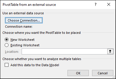
3. In the Create PivotTable dialog box, click From External Data Source.
4. Click Choose Connection.
5. On the Connections tab, in the Show box, keep All Connections selected, or pick the connection category that has the data source you want to connect to.

To reuse or share an existing connection, use a connection from Connections in this Workbook.

1. In the list of connections, select the connection you want, and then click Open.
2. Under Choose where you want the PivotTable report to be placed, pick a location.
   • To place the PivotTable in a new worksheet starting at cell A1, choose New Worksheet.
   • To place the PivotTable in the active worksheet, choose Existing Worksheet, and then in the Location box, enter the cell where you want the PivotTable to start.
3. Click OK.Excel adds an empty PivotTable and shows the Field List so that you can show the fields you want and rearrange them to create your own layout.
4. In the field list section, check the box next to a field name to place the field in a default area of the areas section of the Field List.Typically, nonnumeric fields are added to the Rows area, numeric fields are added to the Values area, and date and time fields are added to the Columns area. You can move fields to a different area as needed.Tip: You can also right-click a field name, and then select Add to Report Filter, Add to Column Labels, Add to Row Labels, or Add to Values to place the field in that area of the areas section, or drag a field from the field section to an area in the areas section.Use the Field List to further design the layout and format of a PivotTable by right-clicking the fields in the areas section, and then selecting the area you want, or by dragging the fields between the areas in the areas section.

Connect to a new external data source

To create a new external data connection to SQL Server and import data into Excel as a table or PivotTable, do the following:

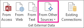
1. Click Data > From Other Sources.
2. Click the connection you want.
   • Click From SQL Server to create a connection to a SQL Server table.
   • Click From Analysis Services to create a connection to a SQL Server Analysis cube.
3. In the Data Connection Wizard, complete the steps to establish the connection.
   • On page 1, enter the database server and specify how you want to log on to the server.
   • On page 2, enter the database, table, or query that contains the data you want.
   • On page 3, enter the connection file you want to create.

To create a new connection to an Access database and import data into Excel as a table or PivotTable, do the following:

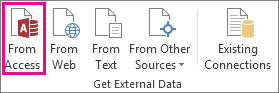
1. Click Data > From Access.
   
   
2. In the Select Data Source dialog box, locate the database you want to connect to, and click Open.
3. In the Select Table dialog box, select the table you want and then click OK.

If there are multiple tables, check the Enable selection of multiple tables box so you can check the boxes of the tables you want, and then click OK.

In the Import Data dialog box, select how you want to view the data in your workbook and where you want to put it, and then click OK.

The tables are automatically added to the Data Model, and the Access database is added to your workbook connections.

Group or ungroup data in a PivotTable

Applies To

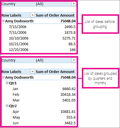
Grouping data in a PivotTable can help you show a subset of data to analyze. For example, you may want to group an unwieldy list date and time fields in the PivotTable into quarters and monthsWindowsMac

Paused

Group data

1. In the PivotTable, right-click a value and select Group.
2. In the Grouping box, select Starting at and Ending at checkboxes, and edit the values if needed.
3. Under By, select a time period. For numerical fields, enter a number that specifies the interval for each group.
4. Select OK.

Group selected items

1. Hold Ctrl and select two or more values.
2. Right-click and select Group.

Group by date and time

With time grouping, relationships across time-related fields are automatically detected and grouped together when you add rows of time fields to your PivotTables. Once grouped together, you can drag the group to your Pivot Table and start your analysis.

Name a group

1. Select the group.
2. Select Analyze > Field Settings. In the PivotTable Analyze tab under Active Field click Field Settings.
3. Change the Custom Name to something you want and then select OK.

Ungroup grouped data

1. Right-click any item that is in the group.
2. Select Ungroup.

Use the Field List to arrange fields in a PivotTable

After you create a PivotTable, you’ll see the Field List. You can change the design of the PivotTable by adding and arranging its fields. If you want to sort or filter the columns of data shown in the PivotTable, see Sort data in a PivotTable and Filter data in a PivotTable. 
 

Use the Field List

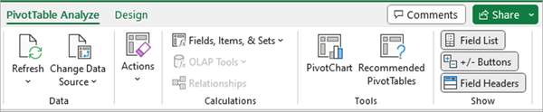
The Field List should appear when you click anywhere in the PivotTable. If you click inside the PivotTable but don’t see the Field List, open it by clicking anywhere in the PivotTable. Then, show the PivotTable Tools on the ribbon and click Analyze> Field List.

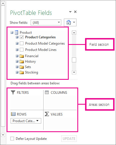
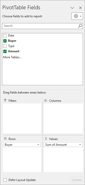
The Field List has a field section in which you pick the fields you want to show in your PivotTable, and the Areas section (at the bottom) in which you can arrange those fields the way you want.

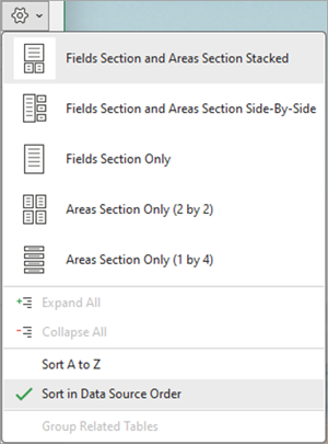
Tip: If you want to change how sections are shown in the Field List, click the Tools button   and then pick the layout you want.

Add, rearrange, and delete fields in the Field List

Use the field section of the Field List to add fields to your PivotTable, by checking the box next to field names to place those fields in the default area of the Field List.

Note: Typically, nonnumeric fields are added to the Rows area, numeric fields are added to the Values area, and Online Analytical Processing (OLAP) date and time hierarchies are added to the Columns area.

Use the areas section (at the bottom) of the Field List to rearrange fields the way you want by dragging them between the four areas.
 

Fields that you place in different areas are shown in the PivotTable as follows:

• Filters area fields are shown as top-level report filters above the PivotTable, like this:
  
  
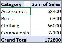
• Columns area fields are shown as Column Labels at the top of the PivotTable, like this:
  
  

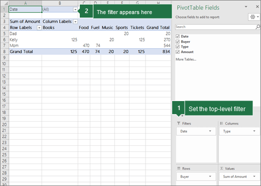
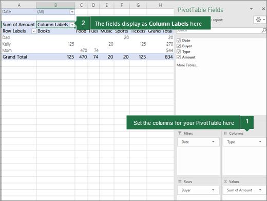
Depending on the hierarchy of the fields, columns may be nested inside columns that are higher in position.

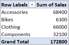
• Rows area fields are shown as Row Labels on the left side of the PivotTable, like this:
  
  

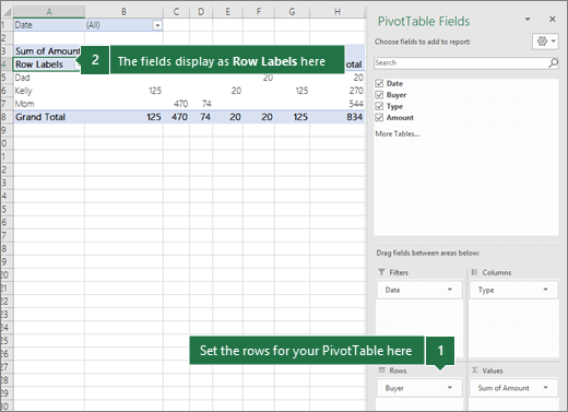
Depending on the hierarchy of the fields, rows may be nested inside rows that are higher in position.

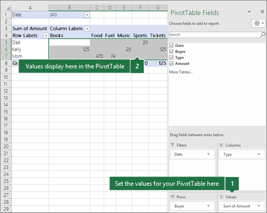
• Values area fields are shown as summarized numeric values in the PivotTable, like this:
  
  

If you have more than one field in an area, you can rearrange the order by dragging the fields into the precise position you want.

To delete a field from the PivotTable, drag the field out of its areas section. You can also remove fields by clicking the down arrow next to the field and then selecting Remove Field.