Calculate the difference between two dates

Applies To

Warning: Excel provides the DATEDIF function in order to support older workbooks from Lotus 1-2-3. The DATEDIF function may calculate incorrect results under certain scenarios. For more information, please go to the known issues section of the DATEDIF function article.

Use the DATEDIF function when you want to calculate the difference between two dates. First put a start date in a cell, and an end date in another. Then type a formula like one of the following.

Note: If the Start_date is greater than the End_date, the result will be #NUM!.

Difference in days

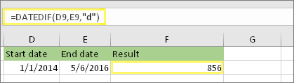
In this example, the start date is in cell D9, and the end date is in E9. The formula is in F9. The “d” returns the number of full days between the two dates.

Difference in weeks

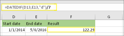
In this example, the start date is in cell D13, and the end date is in E13. The “d” returns the number of days. But notice the /7 at the end. That divides the number of days by 7, since there are 7 days in a week. Note that this result also needs to be formatted as a number. Press CTRL + 1. Then click Number > Decimal places: 2.

Difference in months

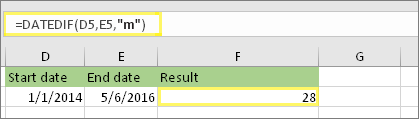
In this example, the start date is in cell D5, and the end date is in E5. In the formula, the “m” returns the number of full months between the two days.

Difference in years

In this example, the start date is in cell D2, and the end date is in E2. The “y” returns the number of full years between the two days.

Calculate age in accumulated years, months, and days

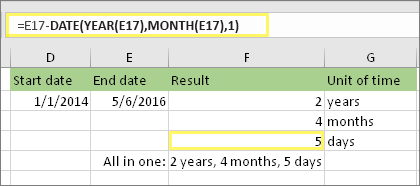
You can also calculate age or someone’s time of service. The result can be something like “2 years, 4 months, 5 days.”

1. Use DATEDIF to find the total years.

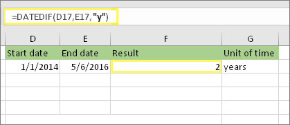
In this example, the start date is in cell D17, and the end date is in E17. In the formula, the “y” returns the number of full years between the two days.

2. Use DATEDIF again with “ym” to find months.

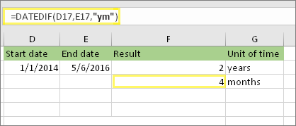
In another cell, use the DATEDIF formula with the “ym” parameter. The “ym” returns the number of remaining months past the last full year.

3. Use a different formula to find days.

Now we need to find the number of remaining days. We’ll do this by writing a different kind of formula, shown above. This formula subtracts the first day of the ending month (5/1/2016) from the original end date in cell E17 (5/6/2016). Here’s how it does this: First the DATE function creates the date, 5/1/2016. It creates it using the year in cell E17, and the month in cell E17. Then the 1 represents the first day of that month. The result for the DATE function is 5/1/2016. Then, we subtract that from the original end date in cell E17, which is 5/6/2016. 5/6/2016 minus 5/1/2016 is 5 days.

Warning: We don’t recommend using the DATEDIF “md” argument because it may calculate inaccurate results.

4. Optional: Combine three formulas in one.

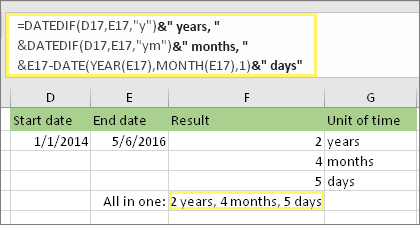
You can put all three calculations in one cell like this example. Use ampersands, quotes, and text. It’s a longer formula to type, but at least it’s all in one. Tip: Press ALT+ENTER to put line breaks in your formula. This makes it easier to read. Also, press CTRL+SHIFT+U if you can’t see the whole formula.

Download our examples

You can download an example workbook with all of the examples in this article. You can follow along, or create your own formulas.

Download date calculation examples

Other date and time calculations

Calculate between today and another date

As you saw above, the DATEDIF function calculates the difference between a start date and an end date. However, instead of typing specific dates, you can also use the TODAY() function inside the formula. When you use the TODAY() function, Excel uses your computer’s current date for the date. Keep in mind this will change when the file is opened again on a future day.

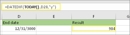
Please note that at the time of this writing, the day was October 6, 2016.

Calculate workdays, with or without holidays

Use the NETWORKDAYS.INTL function when you want to calculate the number of workdays between two dates. You can also have it exclude weekends and holidays too.

Before you begin: Decide if you want to exclude holiday dates. If you do, type a list of holiday dates in a separate area or sheet. Put each holiday date in its own cell. Then select those cells, select Formulas > Define Name. Name the range MyHolidays, and click OK. Then create the formula using the steps below.

1. Type a start date and an end date.

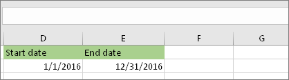
In this example, the start date is in cell D53 and the end date is in cell E53.

2. In another cell, type a formula like this:

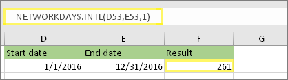
Type a formula like the above example. The 1 in the formula establishes Saturdays and Sundays as weekend days, and excludes them from the total.

3. If necessary, change the 1.

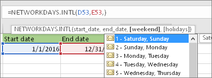
If Saturday and Sunday are not your weekend days, then change the 1 to another number from the IntelliSense list. For example, 2 establishes Sundays and Mondays as weekend days.

4. Type the holiday range name.

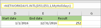
If you created a holiday range name in the “Before you begin” section above, then type it at the end like this. If you don’t have holidays, you can leave the comma and MyHolidays out.

Calculate elapsed time

You can calculate elapsed time by subtracting one time from another. First put a start time in a cell, and an end time in another. Make sure to type a full time, including the hour, minutes, and a space before the AM or PM. Here’s how:

1. Type a start time and end time.

In this example, the start time is in cell D80 and the end time is in E80. Make sure to type the hour, minute, and a space before the AM or PM.

2. Set the h:mm AM/PM format.

Select both dates and press CTRL + 1 (or  + 1 on the Mac). Make sure to select Custom > h:mm AM/PM, if it isn’t already set.

3. Subtract the two times.

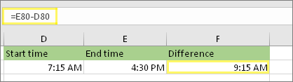
In another cell, subtract the start time cell from the end time cell.

4. Set the h:mm format.

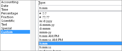
Press CTRL + 1 (or  + 1 on the Mac). Choose Custom > h:mm so that the result excludes AM and PM.

Calculate elapsed time between two dates and times

To calculate the time between two dates and times, you can simply subtract one from the other. However, you must apply formatting to each cell to ensure that Excel returns the result you want.

1. Type two full dates and times.

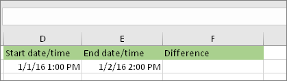
In one cell, type a full start date/time. And in another cell, type a full end date/time. Each cell should have a month, day, year, hour, minute, and a space before the AM or PM.

2. Set the 3/14/12 1:30 PM format.

Select both cells, and then press CTRL + 1 (or  + 1 on the Mac). Then select Date > 3/14/12 1:30 PM. This isn’t the date you’ll set, it’s just a sample of how the format will look. Note that in versions prior to Excel 2016, this format might have a different sample date like 3/14/01 1:30 PM.

3. Subtract the two.

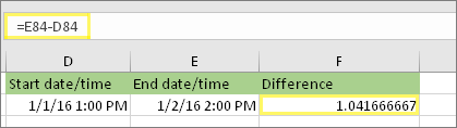
In another cell, subtract the start date/time from the end date/time. The result will probably look like a number and decimal. You’ll fix that in the next step.

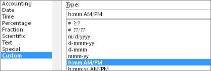
4. Set the [h]:mm format.

Press CTRL + 1 (or  + 1 on the Mac). Select Custom. In the Type box, type [h]:mm.

DATEDIF function

Applies To

Calculates the number of days, months, or years between two dates.

Warning: 

• Excel provides the DATEDIF function in order to support older workbooks from Lotus 1-2-3. The DATEDIF function may calculate incorrect results under certain scenarios. Please see the known issues section of this article for further details.
• Tip: If you want to find the number of days between two dates, simply subtract the later date from the earlier date. This works because dates are stored as numbers in Excel.

Syntax

DATEDIF(start_date,end_date,unit)

Argument	Description
start_date   Required	A date that represents the first, or starting date of a given period. Dates may be entered as text strings within quotation marks (for example, “2001/1/30”), as serial numbers (for example, 36921, which represents January 30, 2001, if you’re using the 1900 date system), or as the results of other formulas or functions (for example, DATEVALUE(“2001/1/30”)).
end_date   Required	A date that represents the last, or ending, date of the period.
Unit	The type of information that you want returned, where:UnitReturns“Y“The number of complete years in the period.”M“The number of complete months in the period.”D“The number of days in the period.”MD“The difference between the days in start_date and end_date. The months and years of the dates are ignored.Important: We don’t recommend using the “MD” argument, as there are known limitations with it. See the known issues section below.”YM“The difference between the months in start_date and end_date. The days and years of the dates are ignored”YD“The difference between the days of start_date and end_date. The years of the dates are ignored.

Remarks

• Dates are stored as sequential serial numbers so they can be used in calculations. By default, January 1, 1900 is serial number 1, and January 1, 2008 is serial number 39448 because it is 39,447 days after January 1, 1900.
• The DATEDIF function is useful in formulas where you need to calculate an age.
• If the start_date is greater than the end_date, the result will be #NUM!.

Examples

Start_date	End_date	Formula	Description (Result)
1/1/2001	1/1/2003	=DATEDIF(Start_date,End_date,”Y”)	Two complete years in the period (2)
6/1/2001	8/15/2002	=DATEDIF(Start_date,End_date,”D”)	440 days between June 1, 2001, and August 15, 2002 (440)
6/1/2001	8/15/2002	=DATEDIF(Start_date,End_date,”YD”)	75 days between June 1 and August 15, ignoring the years of the dates (75)

Known issues

The “MD” argument may result in a negative number, a zero, or an inaccurate result. If you are trying to calculate the remaining days after the last completed month, here is a workaround:

This formula subtracts the first day of the ending month (5/1/2016) from the original end date in cell E17 (5/6/2016). Here’s how it does this: First the DATE function creates the date, 5/1/2016. It creates it using the year in cell E17, and the month in cell E17. Then the 1 represents the first day of that month. The result for the DATE function is 5/1/2016. Then, we subtract that from the original end date in cell E17, which is 5/6/2016. 5/6/2016 minus 5/1/2016 is 5 days.

NETWORKDAYS.INTL function

Applies To

Returns the number of whole workdays between two dates using parameters to indicate which and how many days are weekend days. Weekend days and any days that are specified as holidays are not considered as workdays.

Syntax

NETWORKDAYS.INTL(start_date, end_date, [weekend], [holidays])

The NETWORKDAYS.INTL function syntax has the following arguments:

• Start_date and end_date    Required. The dates for which the difference is to be computed. The start_date can be earlier than, the same as, or later than the end_date.
• Weekend    Optional. Indicates the days of the week that are weekend days and are not included in the number of whole working days between start_date and end_date. Weekend is a weekend number or string that specifies when weekends occur.Weekend number values indicate the following weekend days:

Weekend number	Weekend days
1 or omitted	Saturday, Sunday
2	Sunday, Monday
3	Monday, Tuesday
4	Tuesday, Wednesday
5	Wednesday, Thursday
6	Thursday, Friday
7	Friday, Saturday
11	Sunday only
12	Monday only
13	Tuesday only
14	Wednesday only
15	Thursday only
16	Friday only
17	Saturday only

Weekend string values are seven characters long and each character in the string represents a day of the week, starting with Monday. 1 represents a non-workday and 0 represents a workday. Only the characters 1 and 0 are permitted in the string. Using 1111111 will always return 0.

For example, 0000011 would result in a weekend that is Saturday and Sunday.

• Holidays    Optional. An optional set of one or more dates that are to be excluded from the working day calendar. Holidays shall be a range of cells that contain the dates, or an array constant of the serial values that represent those dates. The ordering of dates or serial values in holidays can be arbitrary.

Remarks

• If start_date is later than end_date, the return value will be negative, and the magnitude will be the number of whole workdays.
• If start_date is out of range for the current date base value, NETWORKDAYS.INTL returns the #NUM! error value.
• If end_date is out of range for the current date base value, NETWORKDAYS.INTL returns the #NUM! error value.
• If a weekend string is of invalid length or contains invalid characters, NETWORKDAYS.INTL returns the #VALUE! error value.

Example

Copy the example data in the following table, and paste it in cell A1 of a new Excel worksheet. For formulas to show results, select them, press F2, and then press Enter. If you need to, you can adjust the column widths to see all the data.

Formula	Description	Result
=NETWORKDAYS.INTL(DATE(2006,1,1),DATE(2006,1,31))	Results in 22 future workdays. Subtracts 9 nonworking weekend days (5 Saturdays and 4 Sundays) from the 31 total days between the two dates. By default, Saturday and Sunday are considered non-working days.	22
=NETWORKDAYS.INTL(DATE(2006,2,28),DATE(2006,1,31))	Results in -21, which is 21 workdays in the past.	-21
=NETWORKDAYS.INTL(DATE(2006,1,1),DATE(2006,2,1),7,{“2006/1/2″,”2006/1/16”})	Results in 22 future workdays by sutracting 10 nonworking days (4 Fridays, 4 Saturdays, 2 Holidays) from the 32 days between Jan 1 2006 and Feb 1 2006. Uses the 7 argument for weekend, which is Friday and Saturday. There are also two holidays in this time period.	22
=NETWORKDAYS.INTL(DATE(2006,1,1),DATE(2006,2,1),”0010001″,{“2006/1/2″,”2006/1/16”})	Results in 22 future workdays. Same time period as example directly above, but with Sunday and Wednesday as weekend days.	20

NETWORKDAYS function

Applies To

This article describes the formula syntax and usage of the NETWORKDAYS function in Microsoft Excel.

Description

Returns the number of whole working days between start_date and end_date. Working days exclude weekends and any dates identified in holidays. Use NETWORKDAYS to calculate employee benefits that accrue based on the number of days worked during a specific term.

Tip:  To calculate whole workdays between two dates by using parameters to indicate which and how many days are weekend days, use the NETWORKDAYS.INTL function.

Syntax

NETWORKDAYS(start_date, end_date, [holidays])

The NETWORKDAYS function syntax has the following arguments:

• Start_date    Required. A date that represents the start date.
• End_date    Required. A date that represents the end date.
• Holidays    Optional. An optional range of one or more dates to exclude from the working calendar, such as state and federal holidays and floating holidays. The list can be either a range of cells that contains the dates or an array constant of the serial numbers that represent the dates.

Important:  Dates should be entered by using the DATE function, or as results of other formulas or functions. For example, use DATE(2012,5,23) for the 23rd day of May, 2012. Problems can occur if dates are entered as text.

Remarks

• Microsoft Excel stores dates as sequential serial numbers so they can be used in calculations. By default, January 1, 1900 is serial number 1, and January 1, 2012 is serial number 40909 because it is 40,909 days after January 1, 1900.
• If any argument is not a valid date, NETWORKDAYS returns the #VALUE! error value.

Example

Copy the example data in the following table, and paste it in cell A1 of a new Excel worksheet. For formulas to show results, select them, press F2, and then press Enter. If you need to, you can adjust the column widths to see all the data.

Date	Description
10/1/2012	Start date of project
3/1/2013	End date of project
11/22/2012	Holiday
12/4/2012	Holiday
1/21/2013	Holiday
Formula	Description	Result
=NETWORKDAYS(A2,A3)	Number of workdays between the start (10/1/2012) and end date (3/1/2013).	110
=NETWORKDAYS(A2,A3,A4)	Number of workdays between the start (10/1/2012) and end date (3/1/2013), with the 11/22/2012 holiday as a non-working day.	109
=NETWORKDAYS(A2,A3,A4:A6)	Number of workdays between the start (10/1/2012) and end date (3/1/2013), with the three holidays as non-working days.	107

Date and time functions (reference)

Applies To

To get detailed information about a function, click its name in the first column.

Function	Description
DATE function	Returns the serial number of a particular date
DATEDIF function	Calculates the number of days, months, or years between two dates. This function is useful in formulas where you need to calculate an age.
DATEVALUE function	Converts a date in the form of text to a serial number
DAY function	Converts a serial number to a day of the month
DAYS function	Returns the number of days between two dates
DAYS360 function	Calculates the number of days between two dates based on a 360-day year
EDATE function	Returns the serial number of the date that is the indicated number of months before or after the start date
EOMONTH function	Returns the serial number of the last day of the month before or after a specified number of months
HOUR function	Converts a serial number to an hour
ISOWEEKNUM function	Returns the number of the ISO week number of the year for a given date
MINUTE function	Converts a serial number to a minute
MONTH function	Converts a serial number to a month
NETWORKDAYS function	Returns the number of whole workdays between two dates
NETWORKDAYS.INTL function	Returns the number of whole workdays between two dates using parameters to indicate which and how many days are weekend days
NOW function	Returns the serial number of the current date and time
SECOND function	Converts a serial number to a second
TIME function	Returns the serial number of a particular time
TIMEVALUE function	Converts a time in the form of text to a serial number
TODAY function	Returns the serial number of today’s date
WEEKDAY function	Converts a serial number to a day of the week
WEEKNUM function	Converts a serial number to a number representing where the week falls numerically with a year
WORKDAY function	Returns the serial number of the date before or after a specified number of workdays
WORKDAY.INTL function	Returns the serial number of the date before or after a specified number of workdays using parameters to indicate which and how many days are weekend days
YEAR function	Converts a serial number to a year
YEARFRAC function	Returns the year fraction representing the number of whole days between start_date and end_date

Important: The calculated results of formulas and some Excel worksheet functions may differ slightly between a Windows PC using x86 or x86-64 architecture and a Windows RT PC using ARM architecture.

Calculate the difference between two times in Excel

Applies To

Let’s say that you want find out how long it takes for an employee to complete an assembly line operation or a fast food order to be processed at peak hours. There are several ways to calculate the difference between two times.

Present the result in the standard time format

There are two approaches that you can take to present the results in the standard time format (hours : minutes : seconds). You use the subtraction operator (–) to find the difference between times, and then do either of the following:

Apply a custom format code to the cell by doing the following:

1. Select the cell.
2. On the Home tab, in the Number group, click the arrow next to the General box, and then click More Number Formats.
3. In the Format Cells dialog box, click Custom in the Category list, and then select a custom format in the Type box.

Use the TEXT function to format the times: When you use the time format codes, hours never exceed 24, minutes never exceed 60, and seconds never exceed 60.

Example Table 1 — Present the result in the standard time format

Use the information in the following table in a blank worksheet and then modify if necessary.

Cell A Example	Cell B Example
Start time	End time
6/9/2007 10:35 AM	6/9/2007 3:30 PM
Formula	Description (Result)
=B2-A2	Hours between two times (4). You must manually apply the custom format “h” to the cell from the Format Cells dialog box.
=B2-A2	Hours and minutes between two times (4:55). You must manually apply the custom format “h:mm” to the cell from the Format Cells dialog box.
=B2-A2	Hours, minutes, and seconds between two times (4:55:00). You must manually apply the custom format “h:mm:ss” to the cell from the Format Cells dialog box.
=TEXT(B2-A2,”h”)	Hours between two times with the cell formatted as “h” by using the TEXT function (4).
=TEXT(B2-A2,”h:mm”)	Hours and minutes between two times with the cell formatted as “h:mm” by using the TEXT function (4:55).
=TEXT(B2-A2,”h:mm:ss”)	Hours, minutes, and seconds between two times with the cell formatted as “h:mm:ss” by using the TEXT function (4:55:00).

Note: If you use both a format applied with the TEXT function and apply a number format to the cell, the TEXT function takes precedence over the cell formatting.

For more information about how to use these functions, see TEXT function and Display numbers as dates or times.

Example Table 2 — Present the result based on a single time unit

To do this task, you’ll use the INT function, or the HOUR, MINUTE, and SECOND functions as shown in the following example.

Use the information in the following table in a blank worksheet and then modify if necessary.

Cell A Example	Cell B Example
Start time	End time
6/9/2007 10:35 AM	6/9/2007 3:30 PM
Formula	Description (Result)
=INT((B2-A2)*24)	Total hours between two times (4)
=(B2-A2)*1440	Total minutes between two times (295)
=(B2-A2)*86400	Total seconds between two times (17700)
=HOUR(B2-A2)	The difference in the hours unit between two times. This value cannot exceed 24 (4).
=MINUTE(B2-A2)	The difference in the minutes unit between two times. This value cannot exceed 60 (55).
=SECOND(B2-A2)	The difference in the seconds unit between two times. This value cannot exceed 60 (0).