Applies To

The IF function is one of the most popular functions in Excel, and it allows you to make logical comparisons between a value and what you expect.

So an IF statement can have two results. The first result is if your comparison is True, the second if your comparison is False.

For example, =IF(C2=”Yes”,1,2) says IF(C2 = Yes, then return a 1, otherwise return a 2).

Paused

Syntax

Simple IF examples

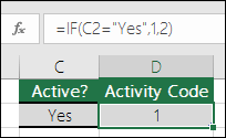
• =IF(C2=”Yes”,1,2)

In the above example, cell D2 says: IF(C2 = Yes, then return a 1, otherwise return a 2)

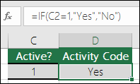
• =IF(C2=1,”Yes”,”No”)

In this example, the formula in cell D2 says: IF(C2 = 1, then return Yes, otherwise return No)As you see, the IF function can be used to evaluate both text and values. It can also be used to evaluate errors. You are not limited to only checking if one thing is equal to another and returning a single result, you can also use mathematical operators and perform additional calculations depending on your criteria. You can also nest multiple IF functions together in order to perform multiple comparisons.

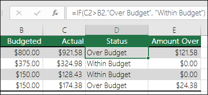
• =IF(C2>B2,”Over Budget”,”Within Budget”)

In the above example, the IF function in D2 is saying IF(C2 Is Greater Than B2, then return “Over Budget”, otherwise return “Within Budget”)

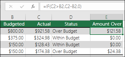
• =IF(C2>B2,C2-B2,0)

In the above illustration, instead of returning a text result, we are going to return a mathematical calculation. So the formula in E2 is saying IF(Actual is Greater than Budgeted, then Subtract the Budgeted amount from the Actual amount, otherwise return nothing).

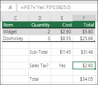
• =IF(E7=”Yes”,F5*0.0825,0)

In this example, the formula in F7 is saying IF(E7 = “Yes”, then calculate the Total Amount in F5 * 8.25%, otherwise no Sales Tax is due so return 0)

Note: If you are going to use text in formulas, you need to wrap the text in quotes (e.g. “Text”). The only exception to that is using TRUE or FALSE, which Excel automatically understands.

Common problems

Problem	What went wrong
0 (zero) in cell	There was no argument for either value_if_true or value_if_False arguments. To see the right value returned, add argument text to the two arguments, or add TRUE or FALSE to the argument.
#NAME? in cell	This usually means that the formula is misspelled.

IF function – nested formulas and avoiding pitfalls

Applies To

The IF function allows you to make a logical comparison between a value and what you expect by testing for a condition and returning a result if True or False.

• =IF(Something is True, then do something, otherwise do something else)

So an IF statement can have two results. The first result is if your comparison is True, the second if your comparison is False.

IF statements are incredibly robust, and form the basis of many spreadsheet models, but they are also the root cause of many spreadsheet issues. Ideally, an IF statement should apply to minimal conditions, such as Male/Female, Yes/No/Maybe, to name a few, but sometimes you might need to evaluate more complex scenarios that require nesting* more than 3 IF functions together.

* “Nesting” refers to the practice of joining multiple functions together in one formula.

Technical details

Use the IF function, one of the logical functions, to return one value if a condition is true and another value if it’s false.

Syntax

IF(logical_test, value_if_true, [value_if_false])

For example:

• =IF(A2>B2,”Over Budget”,”OK”)
• =IF(A2=B2,B4-A4,””)

Argument name	Description
logical_test   (required)	The condition you want to test.
value_if_true   (required)	The value that you want returned if the result of logical_test is TRUE.
value_if_false   (optional)	The value that you want returned if the result of logical_test is FALSE.

Remarks

While Excel will allow you to nest up to 64 different IF functions, it’s not at all advisable to do so. Why?

• Multiple IF statements require a great deal of thought to build correctly and make sure that their logic can calculate correctly through each condition all the way to the end. If you don’t nest your formula 100% accurately, then it might work 75% of the time, but return unexpected results 25% of the time. Unfortunately, the odds of you catching the 25% are slim.
• Multiple IF statements can become incredibly difficult to maintain, especially when you come back some time later and try to figure out what you, or worse someone else, was trying to do.

If you find yourself with an IF statement that just seems to keep growing with no end in sight, it’s time to put down the mouse and rethink your strategy.

Let’s look at how to properly create a complex nested IF statement using multiple IFs, and when to recognize that it’s time to use another tool in your Excel arsenal.

Examples

Following is an example of a relatively standard nested IF statement to convert student test scores to their letter grade equivalent.

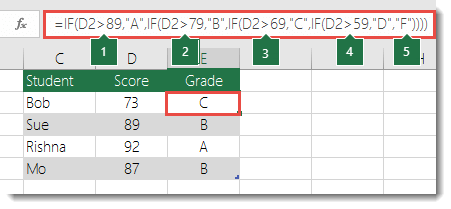
• =IF(D2>89,”A”,IF(D2>79,”B”,IF(D2>69,”C”,IF(D2>59,”D”,”F”))))This complex nested IF statement follows a straightforward logic:

1. If the Test Score (in cell D2) is greater than 89, then the student gets an A
2. If the Test Score is greater than 79, then the student gets a B
3. If the Test Score is greater than 69, then the student gets a C
4. If the Test Score is greater than 59, then the student gets a D
5. Otherwise the student gets an F

This particular example is relatively safe because it’s not likely that the correlation between test scores and letter grades will change, so it won’t require much maintenance. But here’s a thought – what if you need to segment the grades between A+, A and A- (and so on)? Now your four condition IF statement needs to be rewritten to have 12 conditions! Here’s what your formula would look like now:

• =IF(B2>97,”A+”,IF(B2>93,”A”,IF(B2>89,”A-“,IF(B2>87,”B+”,IF(B2>83,”B”,IF(B2>79,”B-“, IF(B2>77,”C+”,IF(B2>73,”C”,IF(B2>69,”C-“,IF(B2>57,”D+”,IF(B2>53,”D”,IF(B2>49,”D-“,”F”))))))))))))

It’s still functionally accurate and will work as expected, but it takes a long time to write and longer to test to make sure it does what you want. Another glaring issue is that you’ve had to enter the scores and equivalent letter grades by hand. What are the odds that you’ll accidentally have a typo? Now imagine trying to do this 64 times with more complex conditions! Sure, it’s possible, but do you really want to subject yourself to this kind of effort and probable errors that will be really hard to spot?

Tip: Every function in Excel requires an opening and closing parenthesis (). Excel will try to help you figure out what goes where by coloring different parts of your formula when you’re editing it. For instance, if you were to edit the above formula, as you move the cursor past each of the ending parentheses “)”, its corresponding opening parenthesis will turn the same color. This can be especially useful in complex nested formulas when you’re trying to figure out if you have enough matching parentheses.

Additional examples

Following is a very common example of calculating Sales Commission based on levels of Revenue achievement.

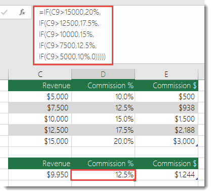
• =IF(C9>15000,20%,IF(C9>12500,17.5%,IF(C9>10000,15%,IF(C9>7500,12.5%,IF(C9>5000,10%,0)))))

This formula says IF(C9 is Greater Than 15,000 then return 20%, IF(C9 is Greater Than 12,500 then return 17.5%, and so on…

While it’s remarkably similar to the earlier Grades example, this formula is a great example of how difficult it can be to maintain large IF statements – what would you need to do if your organization decided to add new compensation levels and possibly even change the existing dollar or percentage values? You’d have a lot of work on your hands!

Tip: You can insert line breaks in the formula bar to make long formulas easier to read. Just press ALT+ENTER before the text you want to wrap to a new line.

Here is an example of the commission scenario with the logic out of order:

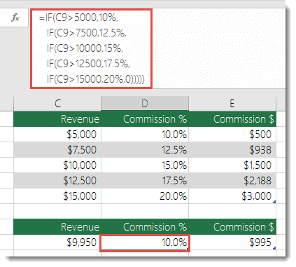
Can you see what’s wrong? Compare the order of the Revenue comparisons to the previous example. Which way is this one going? That’s right, it’s going from bottom up ($5,000 to $15,000), not the other way around. But why should that be such a big deal? It’s a big deal because the formula can’t pass the first evaluation for any value over $5,000. Let’s say you’ve got $12,500 in revenue – the IF statement will return 10% because it is greater than $5,000, and it will stop there. This can be incredibly problematic because in a lot of situations these types of errors go unnoticed until they’ve had a negative impact. So knowing that there are some serious pitfalls with complex nested IF statements, what can you do? In most cases, you can use the VLOOKUP function instead of building a complex formula with the IF function. Using VLOOKUP, you first need to create a reference table:

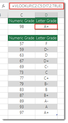
• =VLOOKUP(C2,C5:D17,2,TRUE)

This formula says to look for the value in C2 in the range C5:C17. If the value is found, then return the corresponding value from the same row in column D.

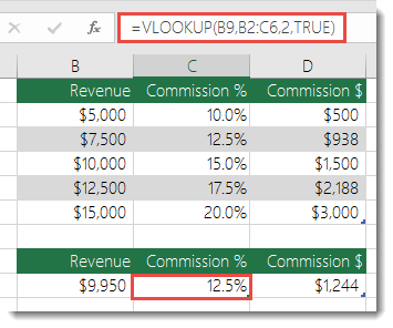
• =VLOOKUP(B9,B2:C6,2,TRUE)

Similarly, this formula looks for the value in cell B9 in the range B2:B22. If the value is found, then return the corresponding value from the same row in column C.

Note: Both of these VLOOKUPs use the TRUE argument at the end of the formulas, meaning we want them to look for an approxiate match. In other words, it will match the exact values in the lookup table, as well as any values that fall between them. In this case the lookup tables need to be sorted in Ascending order, from smallest to largest.

VLOOKUP is covered in much more detail here, but this is sure a lot simpler than a 12-level, complex nested IF statement! There are other less obvious benefits as well:

• VLOOKUP reference tables are right out in the open and easy to see.
• Table values can be easily updated and you never have to touch the formula if your conditions change.
• If you don’t want people to see or interfere with your reference table, just put it on another worksheet.

Did you know?

There is now an IFS function that can replace multiple, nested IF statements with a single function. So instead of our initial grades example, which has 4 nested IF functions:

• =IF(D2>89,”A”,IF(D2>79,”B”,IF(D2>69,”C”,IF(D2>59,”D”,”F”))))

It can be made much simpler with a single IFS function:

• =IFS(D2>89,”A”,D2>79,”B”,D2>69,”C”,D2>59,”D”,TRUE,”F”)

The IFS function is great because you don’t need to worry about all of those IF statements and parentheses.

IFS function

Applies To

The IFS function checks whether one or more conditions are met, and returns a value that corresponds to the first TRUE condition. IFS can take the place of multiple nested IF statements, and is much easier to read with multiple conditions.

Note: This feature is available on Windows or Mac if you have Office 2019, or if you have a Microsoft 365 subscription. If you are a Microsoft 365 subscriber, make sure you have the latest version.

Paused

Simple syntax

Generally, the syntax for the IFS function is:

=IFS([Something is True1, Value if True1,Something is True2,Value if True2,Something is True3,Value if True3)
 

Please note that the IFS function allows you to test up to 127 different conditions. However, we don’t recommend nesting too many conditions with IF or IFS statements. This is because multiple conditions need to be entered in the correct order, and can be very difficult to build, test and update.

Technical details

Example 1

The formula for cells A2:A6 is:

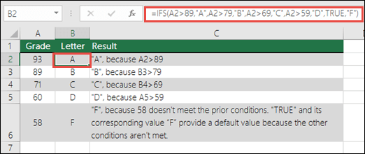
• =IFS(A2>89,”A”,A2>79,”B”,A2>69,”C”,A2>59,”D”,TRUE,”F”)

Which says IF(A2 is Greater Than 89, then return a “A”, IF A2 is Greater Than 79, then return a “B”, and so on and for all other values less than 59, return an “F”).

Example 2

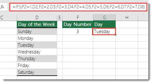
The formula in cell G7 is:

• =IFS(F2=1,D2,F2=2,D3,F2=3,D4,F2=4,D5,F2=5,D6,F2=6,D7,F2=7,D8)

Which says IF(the value in cell F2 equals 1, then return the value in cell D2, IF the value in cell F2 equals 2, then return the value in cell D3, and so on, finally ending with the value in cell D8 if none of the other conditions are met).

Remarks

To specify a default result, enter TRUE for your final logical_test argument. If none of the other conditions are met, the corresponding value will be returned. In Example 1, rows 6 and 7 (with the 58 grade) demonstrate this.

• If a logical_test argument is supplied without a corresponding value_if_true, this function shows a “You’ve entered too few arguments for this function” error message.
• If a logical_test argument is evaluated and resolves to a value other than TRUE or FALSE, this function returns a #VALUE! error.
• If no TRUE conditions are found, this function returns #N/A error.

Using IF with AND, OR, and NOT functions in Excel

Applies To

In Excel, the IF function allows you to make a logical comparison between a value and what you expect by testing for a condition and returning a result if that condition is True or False.

• =IF(Something is True, then do something, otherwise do something else)

But what if you need to test multiple conditions, where let’s say all conditions need to be True or False (AND), or only one condition needs to be True or False (OR), or if you want to check if a condition does NOT meet your criteria? All 3 functions can be used on their own, but it’s much more common to see them paired with IF functions.

Technical Details

Here are overviews of how to structure AND, OR and NOT functions individually. When you combine each one of them with an IF statement, they read like this:

• AND – =IF(AND(Something is True, Something else is True), Value if True, Value if False)
• OR – =IF(OR(Something is True, Something else is True), Value if True, Value if False)
• NOT – =IF(NOT(Something is True), Value if True, Value if False)

Examples

Following are examples of some common nested IF(AND()), IF(OR()) and IF(NOT()) statements in Excel. The AND and OR functions can support up to 255 individual conditions, but it’s not good practice to use more than a few because complex, nested formulas can get very difficult to build, test and maintain. The NOT function only takes one condition.

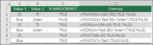
Here are the formulas spelled out according to their logic:

Formula	Description
=IF(AND(A2>0,B2<100),TRUE, FALSE)	IF A2 (25) is greater than 0, AND B2 (75) is less than 100, then return TRUE, otherwise return FALSE. In this case both conditions are true, so TRUE is returned.
=IF(AND(A3=”Red”,B3=”Green”),TRUE,FALSE)	If A3 (“Blue”) = “Red”, AND B3 (“Green”) equals “Green” then return TRUE, otherwise return FALSE. In this case only the first condition is true, so FALSE is returned.
=IF(OR(A4>0,B4<50),TRUE, FALSE)	IF A4 (25) is greater than 0, OR B4 (75) is less than 50, then return TRUE, otherwise return FALSE. In this case, only the first condition is TRUE, but since OR only requires one argument to be true the formula returns TRUE.
=IF(OR(A5=”Red”,B5=”Green”),TRUE,FALSE)	IF A5 (“Blue”) equals “Red”, OR B5 (“Green”) equals “Green” then return TRUE, otherwise return FALSE. In this case, the second argument is True, so the formula returns TRUE.
=IF(NOT(A6>50),TRUE,FALSE)	IF A6 (25) is NOT greater than 50, then return TRUE, otherwise return FALSE. In this case 25 is not greater than 50, so the formula returns TRUE.
=IF(NOT(A7=”Red”),TRUE,FALSE)	IF A7 (“Blue”) is NOT equal to “Red”, then return TRUE, otherwise return FALSE.

Note that all of the examples have a closing parenthesis after their respective conditions are entered. The remaining True/False arguments are then left as part of the outer IF statement. You can also substitute Text or Numeric values for the TRUE/FALSE values to be returned in the examples.

Here are some examples of using AND, OR and NOT to evaluate dates.

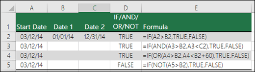
Here are the formulas spelled out according to their logic:

Formula	Description
=IF(A2>B2,TRUE,FALSE)	IF A2 is greater than B2, return TRUE, otherwise return FALSE. 03/12/14 is greater than 01/01/14, so the formula returns TRUE.
=IF(AND(A3>B2,A3<C2),TRUE,FALSE)	IF A3 is greater than B2 AND A3 is less than C2, return TRUE, otherwise return FALSE. In this case both arguments are true, so the formula returns TRUE.
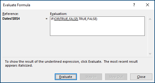
=IF(OR(A4>B2,A4<B2+60),TRUE,FALSE)	IF A4 is greater than B2 OR A4 is less than B2 + 60, return TRUE, otherwise return FALSE. In this case the first argument is true, but the second is false. Since OR only needs one of the arguments to be true, the formula returns TRUE. If you use the Evaluate Formula Wizard from the Formula tab you’ll see how Excel evaluates the formula.
=IF(NOT(A5>B2),TRUE,FALSE)	IF A5 is not greater than B2, then return TRUE, otherwise return FALSE. In this case, A5 is greater than B2, so the formula returns FALSE.

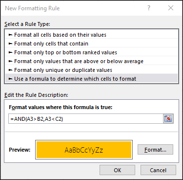
Using AND, OR and NOT with Conditional Formatting in Excel

In Excel, you can also use AND, OR and NOT to set Conditional Formatting criteria with the formula option. When you do this you can omit the IF function and use AND, OR and NOT on their own.

In Excel, from the Home tab, click Conditional Formatting > New Rule. Next, select the “Use a formula to determine which cells to format” option, enter your formula and apply the format of your choice.

Using the earlier Dates example, here is what the formulas would be.

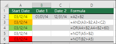
Formula	Description
=A2>B2	If A2 is greater than B2, format the cell, otherwise do nothing.
=AND(A3>B2,A3<C2)	If A3 is greater than B2 AND A3 is less than C2, format the cell, otherwise do nothing.
=OR(A4>B2,A4<B2+60)	If A4 is greater than B2 OR A4 is less than B2 plus 60 (days), then format the cell, otherwise do nothing.
=NOT(A5>B2)	If A5 is NOT greater than B2, format the cell, otherwise do nothing. In this case A5 is greater than B2, so the result will return FALSE. If you were to change the formula to =NOT(B2>A5) it would return TRUE and the cell would be formatted.

Note: A common error is to enter your formula into Conditional Formatting without the equals sign (=). If you do this you’ll see that the Conditional Formatting dialog will add the equals sign and quotes to the formula – =”OR(A4>B2,A4<B2+60)”, so you’ll need to remove the quotes before the formula will respond properly.