Applies To

You can apply formatting to a cell or group of cells and the data therein. You can think of it as a cell being the frame in which the data is held.

 

Format cells

To change cell formatting without using predefined styles, take these steps.  

1. Select a cell or multiple cells. 
2. In the Home ribbon Font area, select from options such as Bold, Font Color, or Font Size. 

Apply Excel Styles 

1. Select the cells.
2. In the Home ribbon Styles area, select Cell Styles. 
3. Select from the available style options.  

Modify an Excel Style

1. Select the cells that have an Excel Style applied.
2. Right-click the applied style in Home > Cell Styles.
3. Select Modify > Format to modify the applied style. 

Create and format tables

Applies To

Create and format a table to visually group and analyze data.

Note: Excel tables shouldn’t be confused with the data tables that are part of a suite of What-If Analysis commands (Forecast, on the Data tab). See Introduction to What-If Analysis for more information.

PausedWindowsmacOSWeb

1. Select a cell within your data.
2. Select Home > Format as Table.
3. Choose a style for your table.
4. In the Create Table dialog box, set your cell range.
5. Mark if your table has headers.
6. Select OK.

Overview of Excel tables

Applies To

To make managing and analyzing a group of related data easier, you can turn a range of cells into an Excel table (previously known as an Excel list).

Note: Excel tables should not be confused with the data tables that are part of a suite of what-if analysis commands. For more information about data tables, see Calculate multiple results with a data table.

Learn about the elements of an Excel table

A table can include the following elements:

• Header row    By default, a table has a header row. Every table column has filtering enabled in the header row so that you can filter or sort your table data quickly. For more information, see Filter data or Sort data.You can turn off the header row in a table. For more information, see Turn Excel table headers on or off.
• Banded rows    Alternate shading or banding in rows helps to better distinguish the data.
• Calculated columns    By entering a formula in one cell in a table column, you can create a calculated column in which that formula is instantly applied to all other cells in that table column. For more information, see Use calculated columns in an Excel table.
• Total row    Once you add a total row to a table, Excel gives you an AutoSum drop-down list to select from functions such as SUM, AVERAGE, and so on. When you select one of these options, the table will automatically convert them to a SUBTOTAL function, which will ignore rows that have been hidden with a filter by default. If you want to include hidden rows in your calculations, you can change the SUBTOTAL function arguments.For more information, also see Total the data in an Excel table.
• Sizing handle    A sizing handle in the lower-right corner of the table allows you to drag the table to the size that you want.For other ways to resize a table, see Resize a table by adding rows and columns.

Create a table

You can create as many tables as you want in a spreadsheet.

To quickly create a table in Excel, do the following:

1. Select the cell or the range in the data.
2. Select Home > Format as Table.
3. Pick a table style.
4. In the Format as Table dialog box, select the checkbox next to My table as headers if you want the first row of the range to be the header row, and then click OK.

Also watch a video on creating a table in Excel.

Working efficiently with your table data

Excel has some features that enable you to work efficiently with your table data:

• Using structured references    Instead of using cell references, such as A1 and R1C1, you can use structured references that reference table names in a formula. For more information, see Using structured references with Excel tables.
• Ensuring data integrity     You can use the built-in data validation feature in Excel. For example, you may choose to allow only numbers or dates in a column of a table. For more information on how to ensure data integrity, see Apply data validation to cells.

Export an Excel table to a SharePoint site

If you have authoring access to a SharePoint site, you can use it to export an Excel table to a SharePoint list. This way other people can view, edit, and update the table data in the SharePoint list. You can create a one-way connection to the SharePoint list so that you can refresh the table data on the worksheet to incorporate changes that are made to the data in the SharePoint list. For more information, see Export an Excel table to SharePoint.

Total the data in an Excel table

Applies ToNewer Windows versionsNewer Mac versionsWeb

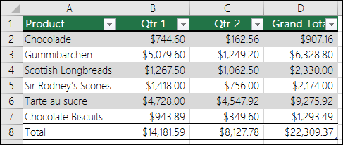
You can quickly total data in an Excel table by enabling the Total Row option, and then use one of several functions that are provided in a drop-down list for each table column. The Total Row default selections use the SUBTOTAL function, which allow you to include or ignore hidden table rows, however you can also use other functions.

Paused

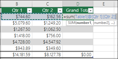
1. Click anywhere inside the table.
2. Go to Table Tools > Design, and select the check box for Total Row.
3. The Total Row is inserted at the bottom of your table.Note: If you apply formulas to a total row, then toggle the total row off and on, Excel will remember your formulas. In the previous example we had already applied the SUM function to the total row. When you apply a total row for the first time, the cells will be empty.
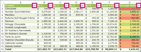
4. Select the column you want to total, then select an option from the drop-down list. In this case, we applied the SUM function to each column:You’ll see that Excel created the following formula: =SUBTOTAL(109,[Midwest]). This is a SUBTOTAL function for SUM, and it is also a Structured Reference formula, which is exclusive to Excel tables. Learn more about Using structured references with Excel tables.You can also apply a different function to the total value, by selecting the More Functions option, or writing your own.Note: If you want to copy a total row formula to an adjacent cell in the total row, drag the formula across using the fill handle. This will update the column references accordingly and display the correct value. If you copy and paste a formula in the total row, it will not update the column references as you copy across, and will result in inaccurate values.

Format an Excel table

Applies ToWindowsWeb

Excel provides numerous predefined table styles that you can use to quickly format a table. If the predefined table styles don’t meet your needs, you can create and apply a custom table style. Although you can delete only custom table styles, you can remove any predefined table style so that it is no longer applied to a table.

You can further adjust the table formatting by choosing Quick Styles options for table elements, such as Header and Total Rows, First and Last Columns, Banded Rows and Columns, as well as Auto Filtering.

Note: The screen shots in this article were taken in Excel 2016. If you have a different version your view might be slightly different, but unless otherwise noted, the functionality is the same.

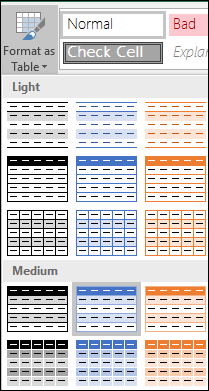
Choose a table style

When you have a data range that is not formatted as a table, Excel will automatically convert it to a table when you select a table style. You can also change the format for an existing table by selecting a different format.

1. Select any cell within the table, or range of cells you want to format as a table.
2. On the Home tab, select Format as Table.
3. Select the table style that you want to use.

Notes: 

• Auto Preview – Excel will automatically format your data range or table with a preview of any style you select but will only apply that style if you press Enter or select with the mouse to confirm it. You can scroll through the table formats with the mouse or your keyboard’s arrow keys.
• When you use Format as Table, Excel automatically converts your data range to a table. If you don’t want to work with your data in a table, you can convert the table back to a regular range while keeping the table style formatting that you applied. For more information, see Convert an Excel table to a range of data.

Create or delete a custom table style

Important: 

• Once created, custom table styles are available from the Table Styles gallery under the Custom section.
• Custom table styles are only stored in the current workbook and are not available in other workbooks.

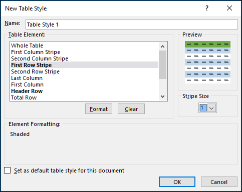
Create a custom table style

1. Select any cell in the table you want to use to create a custom style.
2. On the Home tab, select Format as Table, or expand the Table Styles gallery from the Table Design tab (the Table tab on a Mac).
3. Select New Table Style, which will launch the New Table Style dialog.
4. In the Name box, type a name for the new table style.
5. In the Table Element box, do one of the following:
   • To format an element, select the element, then select Format, and then select the formatting options you want from the Font, Border or Fill tabs.
   • To remove existing formatting from an element, select the element, and then select Clear.
6. Under Preview, you can see how the formatting changes that you made affect the table.
7. To use the new table style as the default table style in the current workbook, select the Set as default table style for this document check box.

Delete a custom table style

1. Select any cell in the table from which you want to delete the custom table style.
2. On the Home tab, select Format as Table, or expand the Table Styles gallery from the Table Design tab (the Table tab on a Mac).
3. Under Custom, right-click the table style that you want to delete, and then select Delete on the shortcut menu.Note: All tables in the current workbook that are using that table style will be displayed in the default table format.

Remove a table style

1. Select any cell in the table from which you want to remove the current table style.
2. On the Home tab, select Format as Table, or expand the Table Styles gallery from the Table Design tab (the Table tab on a Mac).
3. Select Clear.The table will be displayed in the default table format.

Note: Removing a table style does not remove the table. If you don’t want to work with your data in a table, you can convert the table to a regular range. For more information, see Convert an Excel table to a range of data.

Choose table style options to format the table elements

There are several table style options that can be toggled on and off. To apply any of these options:

1. Select any cell in the table.
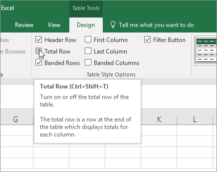
2. Go to Table Design, or the Table tab on a Mac, and in the Table Style Options group, check or uncheck any of the following:
   • Header Row – Apply or remove formatting from the first row in the table.
   • Total Row – Quickly add SUBTOTAL functions like SUM, AVERAGE, COUNT, MIN/MAX to your table from a drop-down selection. SUBTOTAL functions allow you to include or ignore hidden rows in calculations.
   • First Column – Apply or remove formatting from the first column in the table.
   • Last Column – Apply or remove formatting from the last column in the table.
   • Banded Rows – Display odd and even rows with alternating shading for ease of reading.
   • Banded Columns – Display odd and even columns with alternating shading for ease of reading.
   • Filter Button – Toggle AutoFilter on and off.

Resize a table by adding or removing rows and columns in Excel

Applies ToWindowsWeb

After you create an Excel table in your worksheet, you can easily add or remove table rows and columns.

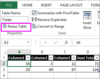
You can use the Resize command in Excel to add rows and columns to a table:

1. Click anywhere in the table, and the Table Design tab appears.
2. Select Table Design > Resize Table.
3. Select the entire range of cells you want your table to include, starting with the upper-most cell.In the example shown below, the original table covers the range A1:C5. After resizing to add two columns and three rows, the table will cover the range A1:E8.Tip: You can also select Collapse Dialog  to temporarily hide the Resize Table dialog box, select the range on the worksheet, and then select Expand dialog .
4. When you’ve selected the range you want for your table, select OK.

Other ways to add rows and columns

Add a row or column to a table by typing in a cell just below the last row or to the right of the last column, by pasting data into a cell, or by inserting rows or columns between existing rows or columns.

Start typing   

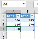
• To add a row at the bottom of the table, start typing in a cell below the last table row. The table expands to include the new row. To add a column to the right of the table, start typing in a cell next to the last table column.

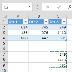
In the example shown below for a row, typing a value in cell A4 expands the table to include that cell in the table along with the adjacent cell in column B.

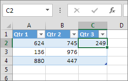
In the example shown below for a column, typing a value in cell C2 expands the table to include column C, naming the table column Qtr 3 because Excel sensed a naming pattern from Qtr 1 and Qtr 2.

Paste data   

• To add a row by pasting, paste your data in the leftmost cell below the last table row. To add a column by pasting, paste your data to the right of the table’s rightmost column.

If the data you paste in a new row has as many or fewer columns than the table, the table expands to include all the cells in the range you pasted. If the data you paste has more columns than the table, the extra columns don’t become part of the table—you need to use the Resize command to expand the table to include them.

In the example shown below for rows, pasting the values from A10:B12 in the first row below the table (row 5) expands the table to include the pasted data.

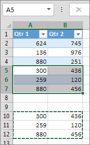
In the example shown below for columns, pasting the values from C7:C9 in the first column to right of the table (column C) expands the table to include the pasted data, adding a heading, Qtr 3.

Use Insert to add a row   

1. To insert a row, pick a cell or row that’s not the header row, and right-click. To insert a column, pick any cell in the table and right-click.
2. Hover over Insert and pick Table Rows Above to insert a new row, or Table Columns to the Left to insert a new column.

If you’re in the last row, you can pick Table Rows Above or Table Rows Below.

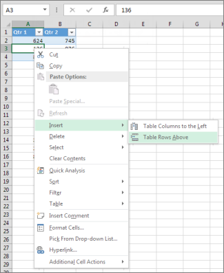
In the example shown below for rows, a row will be inserted above row 3.

For columns, if you have a cell selected in the table’s rightmost column, you can choose between inserting Table Columns to the Left or Table Columns to the Right.

In the example shown below for columns, a column will be inserted to the left of column 1.

Delete rows or columns in a table

1. Select one or more table rows or table columns that you want to delete.You can also just select one or more cells in the table rows or table columns that you want to delete.
2. On the Home tab, in the Cells group, select the arrow next to Delete, and then select Delete Table Rows or Delete Table Columns.You can also right-click one or more rows or columns, hover over Delete on the shortcut menu, and then select Table Columns or Table Rows. Or you can right-click one or more cells in a table row or table column, hover over Delete, and then select Table Rows or Table Columns.

Remove duplicate rows from a table

Just as you can remove duplicates from any selected data in Excel, you can easily remove duplicates from a table.

1. Click anywhere in the table.This displays the Table Design tab.
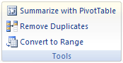
2. On the Table Design tab, in the Tools group, select Remove Duplicates.
3. In the Remove Duplicates dialog box, under Columns, select the columns that contain duplicates that you want to remove.You can also select Unselect All and then select the columns that you want or select Select All to select all of the columns.

Note: Duplicates that you remove are deleted from the worksheet. If you inadvertently delete data that you meant to keep, you can use Ctrl+Z or select Undo  on the Quick Access Toolbar to restore the deleted data. You may also want to use conditional formats to highlight duplicate values before you remove them. For more information, see Add, change, or clear conditional formats.

Remove blank rows from a table

1. Make sure that the active cell is in a table column.
2. Select the arrow  in the column header.
3. To filter for blanks, in the AutoFilter menu at the top of the list of values, clear (Select All), and then at the bottom of the list of values, select (Blanks).Note: The (Blanks) check box is available only if the range of cells or table column contains at least one blank cell.
4. Select the blank rows in the table, and then press CTRL+- (hyphen).

You can use a similar procedure for filtering and removing blank worksheet rows. For more information about how to filter for blank rows in a worksheet, see Filter data in a range or table.

Filter data in a range or table in Excel

Applies To

Use AutoFilter or built-in comparison operators like “greater than” and “top 10” in Excel to show the data you want and hide the rest. Once you filter data in a range of cells or table, you can either reapply a filter to get up-to-date results, or clear a filter to redisplay all of the data.WindowsWebmacOS

Use filters to temporarily hide some of the data in a table, so you can focus on the data you want to see.

Paused

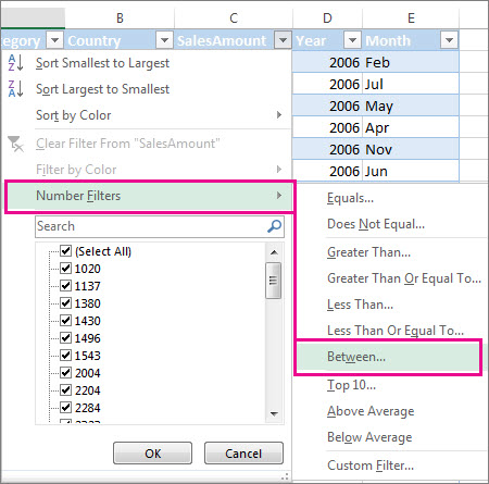
Filter a range of data

1. Select any cell within the range.
2. Select Data > Filter.
3. Select the column header arrow .
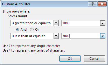
4. Select Text Filters or Number Filters, and then select a comparison, like Between.
5. Enter the filter criteria and select OK.

Filter data in a table

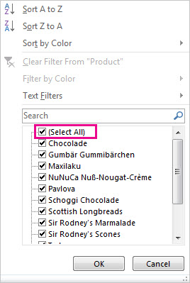
When you put your data in a table, filter controls are automatically added to the table headers.

1. Select the column header arrow  for the column you want to filter.
2. Uncheck (Select All) and select the boxes you want to show.
3. Select OK.The column header arrow  changes to a Filter icon. Select this icon to change or clear the filter.

Convert an Excel table to a range of data

Applies To

After you create an Excel table, you may only want the table style without the table functionality. To stop working with your data in a table without losing any table style formatting that you applied, you can convert the table to a regular range of data on the worksheet.

Important: In order to convert to a range, you must have an Excel table to start with. For more information, see Create or delete an Excel table.WindowsMacWeb

1. Click anywhere in the table and then go to Table Design on the Ribbon.
2. In the Tools group, select Convert to Range.-OR-Right-click the table, then in the shortcut menu, select Table > Convert to Range.Note: Table features are no longer available after you convert the table back to a range. For example, the row headers no longer include the sort and filter arrows, and structured references (references that use table names) that were used in formulas turn into regular cell references.

Using structured references with Excel tables

Applies To

When you create an Excel table, Excel assigns a name to the table, and to each column header in the table. When you add formulas to an Excel table, those names can appear automatically as you enter the formula and select the cell references in the table instead of manually entering them. Here’s an example of what Excel does:

Instead of using explicit cell references	Excel uses table and column names
=Sum(C2:C7)	=SUM(DeptSales[Sales Amount])

That combination of table and column names is called a structured reference. The names in structured references adjust whenever you add or remove data from the table.

Structured references also appear when you create a formula outside of an Excel table that references table data. The references can make it easier to locate tables in a large workbook.

To include structured references in your formula, select the table cells you want to reference instead of typing their cell reference in the formula. Let’s use the following example data to enter a formula that automatically uses structured references to calculate the amount of a sales commission.

Sales Person	Region	Sales Amount	% Commission	Commission Amount
Joe	North	260	10%
Robert	South	660	15%
Michelle	East	940	15%
Erich	West	410	12%
Dafna	North	800	15%
Rob	South	900	15%

1. Copy the sample data in the table above, including the column headings, and paste it into cell A1 of a new Excel worksheet.
2. To create the table, select any cell within the data range, and press Ctrl+T.
3. Make sure the My table has headers box is checked, and select OK.
4. In cell E2, type an equal sign (=), and select cell C2.In the formula bar, the structured reference [@[Sales Amount]] appears after the equal sign.
5. Type an asterisk (*) directly after the closing bracket, and select cell D2.In the formula bar, the structured reference [@[% Commission]] appears after the asterisk.
6. Press Enter.Excel automatically creates a calculated column and copies the formula down the entire column for you, adjusting it for each row.

What happens when I use explicit cell references?

If you enter explicit cell references in a calculated column, it can be harder to see what the formula is calculating.

1. In your sample worksheet, select cell E2
2. In the formula bar, enter =C2*D2 and press Enter.

Notice that while Excel copies your formula down the column, it doesn’t use structured references. If, for example, you add a column between the existing columns C and D, you’d have to revise your formula.

How do I change a table name?

When you create an Excel table, Excel creates a default table name (Table1, Table2, and so on), but you can change the table name to make it more meaningful.

1. Select any cell in the table to show the Table Design tab on the ribbon.
2. Type the name you want in the Table Name box, and press Enter.

In our example data, we used the name DeptSales.

Use the following rules for table names:

• Use valid characters Always start a name with a letter, an underscore character (_), or a backslash (\). Use letters, numbers, periods, and underscore characters for the rest of the name. You can’t use “C”, “c”, “R”, or “r” for the name, because they’re already designated as a shortcut for selecting the column or row for the active cell when you enter them in the Name or Go To box.

• Don’t use cell references Names can’t be the same as a cell reference, such as Z$100 or R1C1.
• Don’t use a space to separate words Spaces can’t be used in the name. You can use the underscore character (_) and period (.) as word separators. For example, DeptSales, Sales_Tax or First.Quarter.
• Use no more than 255 characters A table name can have up to 255 characters.
• Use unique table names Duplicate names aren’t allowed. Excel doesn’t distinguish between upper and lowercase characters in names so if you enter “Sales” but already have another name called “SALES” in the same workbook, you’ll be prompted to choose a unique name.
• Use an object identifier If you plan on having a mix of tables, PivotTables and charts, it’s a good idea to prefix your names with the object type. For example: tbl_Sales for a sales table, pt_Sales for a sales PivotTable, and chrt_Sales for a sales chart, or ptchrt_Sales for a sales PivotChart. This keeps all of your names in an ordered list in the Name Manager.

Structured reference syntax rules

You can also enter or change structured references manually in the formula but to do that, it will help to understand structured reference syntax. Let’s go over the following formula example:

=SUM(DeptSales[[#Totals],[Sales Amount]],DeptSales[[#Data],[Commission Amount]])

This formula has the following structured reference components:

• Table name:    DeptSales is a custom table name. It references the table data, without any header or total rows. You can use a default table name, such as Table1, or change it to use a custom name.
• Column specifier:    [Sales Amount] and [Commission Amount] are column specifiers that use the names of the columns they represent. They reference the column data, without any column header or total row. Always enclose specifiers in brackets as shown.
• Item specifier:    [#Totals] and [#Data] are special item specifiers that refer to specific portions of the table, such as the total row.
• Table specifier:    [[#Totals],[Sales Amount]] and [[#Data],[Commission Amount]] are table specifiers that represent the outer portions of the structured reference. Outer references follow the table name, and you enclose them in square brackets.
• Structured reference:    (DeptSales[[#Totals],[Sales Amount]] and DeptSales[[#Data],[Commission Amount]] are structured references, represented by a string that begins with the table name and ends with the column specifier.

To create or edit structured references manually, use these syntax rules:

• Use brackets around specifiers    All table, column, and special item specifiers need to be enclosed in matching brackets ([ ]). A specifier that contains other specifiers requires outer matching brackets to enclose the inner matching brackets of the other specifiers. For example: =DeptSales[[Sales Person]:[Region]]
• All column headers are text strings    But they don’t require quotes when they’re used in a structured reference. Numbers or dates, such as 2014 or 1/1/2014, are also considered text strings. You can’t use expressions with column headers. For example, the expression DeptSalesFYSummary[[2014]:[2012]] won’t work.

Use brackets around column headers with special characters    If there are special characters, the entire column header needs to be enclosed in brackets, which means that double brackets are required in a column specifier. For example: =DeptSalesFYSummary[[Total $ Amount]]

Here’s the list of special characters that need extra brackets in the formula:

• Tab
• Line feed
• Carriage return
• Comma (,)
• Colon (:)
• Period (.)
• Left bracket ([)
• Right bracket (])
• Pound sign (#)
• Single quotation mark (‘)
• Double quotation mark (“)
• Left brace ({)
• Right brace (})
• Dollar sign ($)
• Caret (^)
• Ampersand (&)
• Asterisk (*)
• Plus sign (+)
• Equal sign (=)
• Minus sign (-)
• Greater than symbol (>)
• Less than symbol (<)
• Division sign (/)
• At sign (@)
• Backslash (\)
• Exclamation point (!)
• Left parenthesis (()
• Right parenthesis ())
• Percent sign (%)
• Question mark (?)
• Backtick (`)
• Semicolon (;)
• Tilde (~)
• Underscore (_)
• Use an escape character for some special characters in column headers    Some characters have special meaning and require the use of a single quotation mark (‘) as an escape character. For example: =DeptSalesFYSummary[‘#OfItems]

Here’s the list of special characters that need an escape character (‘) in the formula:

• Left bracket ([)
• Right bracket (])
• Pound sign (#)
• Single quotation mark (‘)
• At sign (@)

Use the space character to improve readability in a structured reference    You can use space characters to improve the readability of a structured reference. For example: =DeptSales[ [Sales Person]:[Region] ] or =DeptSales[[#Headers], [#Data], [% Commission]]

It’s recommended to use one space:

• After the first left bracket ([)
• Preceding the last right bracket (]).
• After a comma.

Reference operators

For more flexibility in specifying ranges of cells, you can use the following reference operators to combine column specifiers.

This structured reference:	Refers to:	By using the:	Which is cell range:
=DeptSales[[Sales Person]:[Region]]	All of the cells in two or more adjacent columns	: (colon) range operator	A2:B7
=DeptSales[Sales Amount],DeptSales[Commission Amount]	A combination of two or more columns	, (comma) union operator	C2:C7, E2:E7
=DeptSales[[Sales Person]:[Sales Amount]] DeptSales[[Region]:[% Commission]]	The intersection of two or more columns	(space) intersection operator	B2:C7

Special item specifiers

To refer to specific portions of a table, such as just the totals row, you can use any of the following special item specifiers in your structured references.

This special item specifier:	Refers to:
#All	The entire table, including column headers, data, and totals (if any).
#Data	Just the data rows.
#Headers	Just the header row.
#Totals	Just the total row. If none exists, then it returns null.
#This Rowor@or@[Column Name]	Just the cells in the same row as the formula. These specifiers can’t be combined with any other special item specifiers. Use them to force implicit intersection behavior for the reference or to override implicit intersection behavior and refer to single values from a column.Excel automatically changes #This Row specifiers to the shorter @ specifier in tables that have more than one row of data. But if your table has only one row, Excel doesn’t replace the #This Row specifier, which may cause unexpected calculation results when you add more rows. To avoid calculation problems, make sure you enter multiple rows in your table before you enter any structured reference formulas.

Qualifying structured references in calculated columns

When you create a calculated column, you often use a structured reference to create the formula. This structured reference can be unqualified or fully qualified. For example, to create the calculated column, called Commission Amount, that calculates the amount of commission in dollars, you can use the following formulas:

Type of structured reference	Example	Comment
Unqualified	=[Sales Amount]*[% Commission]	Multiplies the corresponding values from the current row.
Fully qualified	=DeptSales[Sales Amount]*DeptSales[% Commission]	Multiples the corresponding values for each row for both columns.

The general rule to follow is this: If you’re using structured references within a table, such as when you create a calculated column, you can use an unqualified structured reference, but if you use the structured reference outside of the table, you need to use a fully qualified structured reference.

Examples of using structured references

Here are some ways to use structured references.

This structured reference:	Refers to:	Which is cell range:
=DeptSales[[#All],[Sales Amount]]	All the cells in the Sales Amount column.	C1:C8
=DeptSales[[#Headers],[% Commission]]	The header of the % Commission column.	D1
=DeptSales[[#Totals],[Region]]	The total of the Region column. If there is no Totals row, then it returns null.	B8
=DeptSales[[#All],[Sales Amount]:[% Commission]]	All the cells in Sales Amount and % Commission.	C1:D8
=DeptSales[[#Data],[% Commission]:[Commission Amount]]	Just the data of the % Commission and Commission Amount columns.	D2:E7
=DeptSales[[#Headers],[Region]:[Commission Amount]]	Just the headers of the columns between Region and Commission Amount.	B1:E1
=DeptSales[[#Totals],[Sales Amount]:[Commission Amount]]	The totals of the Sales Amount through Commission Amount columns. If there is no Totals row, then it returns null.	C8:E8
=DeptSales[[#Headers],[#Data],[% Commission]]	Just the header and the data of % Commission.	D1:D7
=DeptSales[[#This Row], [Commission Amount]]or=DeptSales[@Commission Amount]	The cell at the intersection of the current row and the Commission Amount column. If used in the same row as a header or total row, this will return a #VALUE! error.If you type the longer form of this structured reference (#This Row) in a table with multiple rows of data, Excel automatically replaces it with the shorter form (@). They both work the same.	E5 (if the current row is 5)

Strategies for working with structured references

Consider the following when you work with structured references.

• Use Formula AutoComplete    You may find that using Formula AutoComplete is very useful when you enter structured references and to ensure the use of correct syntax. For more information, see Use Formula AutoComplete.
• Decide whether to generate structured references for tables in semi-selections    By default, when you create a formula, selecting a cell range within a table semi-selects the cells and automatically enters a structured reference instead of the cell range in the formula. This semi-selection behavior makes it much easier to enter a structured reference. You can turn this behavior on or off by selecting or clearing the Use table names in formulas check box in the File > Options > Formulas > Working with formulas dialog.
• Use workbooks with external links to Excel tables in other workbooks    If a workbook contains an external link to an Excel table in another workbook, that linked source workbook must be open in Excel to avoid #REF! errors in the destination workbook that contains the links. If you open the destination workbook first and #REF! errors appear, they will be resolved if you then open the source workbook. If you open the source workbook first, you should see no error codes.
• Convert a range to a table and a table to a range    When you convert a table to a range, all cell references change to their equivalent absolute A1 style references. When you convert a range to a table, Excel doesn’t automatically change any cell references of this range to their equivalent structured references.
• Turn off column headers    You can toggle table column headers on and off from the Table Design tab > Header Row. If you turn off table column headers, structured references that use column names aren’t affected, and you can still use them in formulas. Structured references that refer directly to the table headers (e.g. =DeptSales[[#Headers],[%Commission]]) will result in #REF.
• Add or delete columns and rows to the table    Because table data ranges often change, cell references for structured references adjust automatically. For example, if you use a table name in a formula to count all the data cells in a table, and you then add a row of data, the cell reference automatically adjusts.
• Rename a table or column    If you rename a column or table, Excel automatically changes the use of that table and column header in all structured references that are used in the workbook.
• Move, copy, and fill structured references    All structured references remain the same when you copy or move a formula that uses a structured reference.Note: Copying a structured reference and doing a fill of a structured reference are not the same thing. When you copy, all the structured references remain the same, while when you fill a formula, fully qualified structured references adjust the column specifiers like a series as summarized in the following table.

If the fill direction is:	And while filling, you press:	Then:
Up or down	Nothing	There is no column specifier adjustment.
Up or down	Ctrl	Column specifiers adjust like a series.
Right or left	None	Column specifiers adjust like a series.
Up, down, right, or left	Shift	Instead of overwriting values in current cells, current cell values are moved, and column specifiers are inserted.

Export an Excel table to SharePoint

Applies To

You can export data from an Excel table to a SharePoint list. When you export the list, Excel will create a new SharePoint list on the site. You can then work with the data on the site, just like you would for any other SharePoint list.

Note: Exporting a table as a list does not create a data connection to the SharePoint list. If you were to update the table in Excel after exporting it, the updates will not be reflected in the SharePoint list.

To export a table in an Excel spreadsheet to a list on a SharePoint site, you need:

• A SharePoint site where you are creating the list.
• Permissions to create lists on the site. If you are not sure, contact your SharePoint site administrator.

To view the list in datasheet view on the SharePoint site you need:

• Excel or Access. These programs are required for using the datasheet view on the SharePoint site.Note: Datasheet view is not supported in 64-bit version of Microsoft Office. It is recommended that you install 32-bit version of Office in order to be able to use Datasheet view in a list on a SharePoint site.

Export a table to a SharePoint list

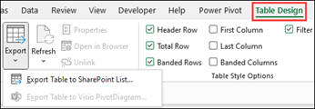
1. Click inside the table.
2. Click Table Design > Export > Export Table to SharePoint List.
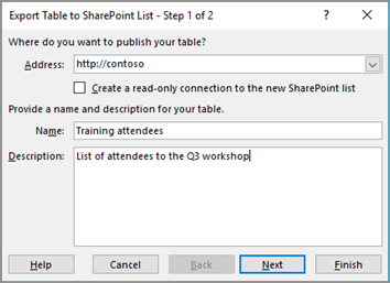
3. In the Address box, type the address, or URL of the SharePoint site.Important: Type everything that’s in your Web address before the “/default.aspx”. For example, if the address is http://contoso/default.aspx, type http://contoso. If the address is http://contoso/teams/accounting/sitepages/home.aspx, type http://contoso/teams/accounting.
4. In the Name box, type a unique name for the list.
5. Optionally, enter a description in the Description box.
6. Click Next.Note: You may be asked to enter your Microsoft 365 credentials, or organizational domain credentials, or both.
7. Review the information given in Columns and Data Types and then click Finish.
8. Click OK.

A message indicating that your table is published, along with the Uniform Resource Locator (URL) appears. Click on the URL to go to the list. Add the URL as a favorite in your browser.

Note: Another way to open the list is to go the SharePoint site, click the gear icon on the upper-right corner, and click Site Contents.

Supported data types

Some Excel data types cannot be exported to a list on the SharePoint site. When unsupported data types are exported, these data types are converted to data types that are compatible with SharePoint lists. For example, formulas that you create in Excel are converted to values in a SharePoint list. After the data is converted, you can create formulas for the columns on the SharePoint site.

When you export an Excel table to a SharePoint site, each column in a SharePoint list is assigned one of the following data types:

• Text (single line)
• Text (multiple lines)
• Currency
• Date/time
• Number
• Hyperlink (URL)

If a column has cells with different data types, Excel applies a data type that can be used for all of the cells in the column. For example, if a column contains numbers and text, the data type in the SharePoint list will be text.