Applies To

Excel for Microsoft 365 Excel for the web Excel 2024 Excel 2021 Excel 2019 Excel 2016

Insert and delete rows and columns to organize your worksheet better.

Note: Microsoft Excel has the following column and row limits: 16,384 columns wide by 1,048,576 rows tall.

Insert or delete a column

Select any cell within the column, then go to Home > Insert > Insert Sheet Columns or Delete Sheet Columns.
Alternatively, right-click the top of the column, and then select Insert or Delete.

Insert or delete a row

Select any cell within the row, then go to Home > Insert > Insert Sheet Rows or Delete Sheet Rows.
Alternatively, right-click the row number, and then select Insert or Delete.

Formatting options

When you select a row or column that has formatting applied, that formatting will be transferred to a new row or column that you insert. If you don’t want the formatting to be applied, you can select the Insert Options button after you insert, and choose from one of the options as follows:

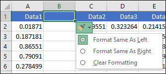
Image of the Insert Options button that's displayed after inserting rows or columns.

If the Insert Options button isn’t visible, then go to File > Options > Advanced > in the Cut, copy and paste group, check the Show Insert Options buttons option.eft-to-right languages, or the upper-right cell for right-to-left languages) appear in the merged cell. The contents of the other cells that you merge are deleted.
Unmerge cells
1.Select the Merge & Center down arrow.
2.Select Unmerge Cells.

Important:

You cannot split an unmerged cell. If you’re looking for information about how to split the contents of an unmerged cell across multiple cells, see Distribute the contents of a cell into adjacent columns.
After merging cells, you can split a merged cell into separate cells again. If you don’t remember where you have merged cells, you can use the Find command to locate merged cells quickly.

Collaborate on Excel workbooks at the same time with co-authoring

You and your colleagues can open and work on the same Excel workbook. This is called co-authoring. When you co-author, you can see each other’s changes quickly—in a matter of seconds. And with certain versions of Excel, you’ll see other people’s selections in different colors. If you’re using a version of Excel that supports co-authoring, you can select Share in the upper-right corner, type email addresses, and then choose a cloud location. But if you need more details, like which versions are supported and where the file can be stored, this article will walk you through the process.WindowsmacOSWebAndroidiOS

Note: This feature is only available if you have a Microsoft 365 subscription. If you are a Microsoft 365subscriber, make sure you have the latest version of Office.

To co-author in Excel for Windows desktops, you need to make sure certain things are set up before you start. After that, it just takes a few steps to co-author with other people.

What you need to co-author

You need a Microsoft 365 subscription.
You need the latest version of Excel for Microsoft 365 installed. Note that if you have a work or school account, you might not have a version that supports co-authoring yet. This might be because your administrator hasn’t provided the latest version to install.
You need to sign in to Microsoft 365 with your subscription account.
You need to use Excel Workbooks in .xlsx, .xlsm, or .xlsb file format. If your file isn’t in this format, open the file and then select File > Save As > Browse > Save as type. Change the format to Excel Workbook (*.xlsx). Note that co-authoring does not support the Strict Open XML Spreadsheet format.

Step 1: Upload the workbook

Using a web browser, upload or create a new workbook on OneDrive, OneDrive for Business, or a SharePoint Online library. Note that SharePoint On-Premises sites (sites that are not hosted by Microsoft) do not support co-authoring. If you aren’t sure which one you’re using, ask the person in charge of your site, or your IT department.

Step 2: Share it

If you uploaded the file, select the filename to open it. The workbook will open in a new tab in your web browser.
Select the Open in Desktop App button.
When the file opens in the Excel desktop app, you may see a yellow bar which says the file is in Protected View. Select the Enable Editing button if that’s the case.
Select Share in the upper-right corner.
By default, all recipients will be able to edit the workbook, however, you can change the settings by selecting the can edit option.
Type email addresses in the address box, and separate each with a semicolon.
Add a message for your recipients. This step is optional.
Select Send.

Note: If you want to send the link yourself, don’t select the Send button. Instead, select Copy link at the bottom of the pane.

Step 3: Other people can open it

If you selected the Share button, people will receive an email message inviting them to open the file. They can select the link to open the workbook. A web browser may open, and the workbook may open in Excel for the web. If they want to use the Excel desktop app to co-author, they can select Edit in Desktop App. However, they’ll need a version of the Excel app that supports co-authoring. Excel for Android, Excel for iOS, Excel Mobile, and Excel for Microsoft 365 subscribers are the versions that currently support co-authoring. If they don’t have a supported version, they can edit in the browser.

Note: If they’re using the latest version of Excel, PowerPoint, or Word there’s an easier way—they can select File > Open and select Shared with Me.

Step 4: Co-author with others

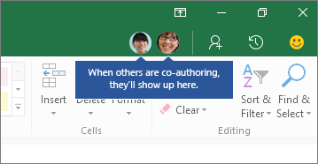
With the file still open in Excel, make sure that AutoSave is on in the upper-left corner. When others eventually open the file, you’ll be co-authoring together. You know you’re co-authoring if you see pictures of people in the upper-right of the Excel window. (You may also see their initials, or a “G” which stands for guest.)

People icons, When others are co-authoring, they'll show up here

Co-authoring tips:

You might see other people’s selections in different colors. This happens if they’re using Excel for Microsoft 365 subscribers, Excel for the web, Excel for Android, Excel Mobile, or Excel for iOS. If they’re using another version, you won’t see their selections, but their changes will appear as they’re working.
If you see other people’s selections in different colors, they’ll show up as blue, purple and so on. However, your selection will always be green. And on other people’s screens, their own selections will be green as well. If you lose track of who’s who, rest your cursor over the selection, and the person’s name will be revealed. If you want to jump to where someone is working, select their picture or initials, and then select the Go to option.

To prevent others from accessing data in your Excel files, protect your Excel file with a password.

Note: This topic covers file-level protection only, and not workbook or worksheet protection. To learn the difference between protecting your Excel file, workbook, or a worksheet, see Protection and security in Excel .

Select File > Info .
Select the Protect Workbook box and choose Encrypt with Password.
Enter a password in the Password box, and then select OK .
Confirm the password in the Reenter Password box, and then select OK .

Warning:

Microsoft cannot retrieve forgotten passwords, so be sure that your password is especially memorable.
There are no restrictions on the passwords you use with regards to length, characters or numbers, but passwords are case-sensitive.
It’s not always secure to distribute password-protected files that contain sensitive information such as credit card numbers.
Be cautious when sharing files or passwords with other users. You still run the risk of passwords falling into the hands of unintended users. Remember that locking a file with a password does not necessarily protect your file from malicious intent.

To prevent other users from viewing hidden worksheets, adding, moving, deleting, or hiding worksheets, and renaming worksheets, you can protect the structure of your Excel workbook with a password.

Notes: Protecting the workbook is not the same as protecting an Excel file or a worksheet with a password. See below for more information:

To lock your file so that other users can’t open it, see Protect an Excel file.
To protect certain areas of the data in your worksheet from other users, you have to protect your worksheet. For more information, see Protect a worksheet.
To know the difference between protecting your Excel file, workbook, or a worksheet, see Protection and security in Excel.

Protect the workbook structure

To protect the structure of your workbook, follow these steps:

Protect Workbook Dialog Box

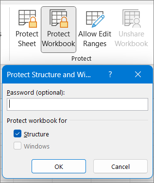
Click Review > Protect Workbook.
Enter a password in the Password box.Important: The password is optional. If you do not supply a password, any user can unprotect and change the workbook. If you do enter a password, make sure that you choose a password that is easy to remember. Write your passwords down and store them someplace safe. If you lose them, Excel cannot recover them for you.
Select OK, re-enter the password to confirm it, and then select OK again.

How can I tell if a workbook is protected?

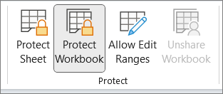
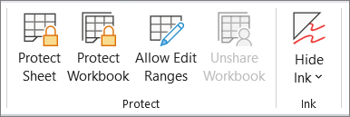
On the Review tab , see the Protect Workbook icon. If it’s highlighted, then the workbook is protected. Protect Workbook Highlighted

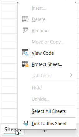
If you click on the bottom of a sheet inside your workbook, you will notice that the options to change the workbook structure, such as Insert, Delete, Rename, Move, Copy, Hide, and Unhide sheets are all unavailable.

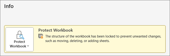
Functions will be unavailable when workbook protection is enabled

The Protect Workbook option in the Info menu also indicates that the workbook’s structure is protected. To view this option, click File > Info > Protect Workbook.

Protect Workbook under the Info menu

Unprotect an Excel workbook

Click Review > Protect Workbook. Enter the password and then click OK.

Protect a worksheet

Applies To

To prevent other users from accidentally or deliberately changing, moving, or deleting data in a worksheet, you can lock the cells on your Excel worksheet and then protect the sheet with a password. Say you own the team status report worksheet, where you want team members to add data in specific cells only and not be able to modify anything else. With worksheet protection, you can make only certain parts of the sheet editable and users will not be able to modify data in any other region in the sheet.

Important: Worksheet level protection isn’t intended as a security feature. It simply prevents users from modifying locked cells within the worksheet. Protecting a worksheet is not the same as protecting an Excel file or a workbook with a password. See below for more information:

To lock your file so that other users can’t open it, see Protect an Excel file.
To prevent users from adding, modifying, moving, copying, or hiding/unhiding sheets within a workbook, see Protect a workbook.
To know the difference between protecting your Excel file, workbook, or a worksheet see Protection and security in Excel.
Worksheet protection is not available for U.S. Government Community Cloud High (GCCH) or Department of Defense (DOD) environments.

WindowsWeb

The following sections describe how to protect and unprotect a worksheet in Excel for Windows.

Choose what cell elements to lock

Here’s what you can lock in an unprotected sheet:

Formulas: If you don’t want other users to see your formulas, you can hide them from being seen in cells or the Formula bar. For more information, see Display or hide formulas.
Ranges: You can enable users to work in specific ranges within a protected sheet. For more information, see Lock or unlock specific areas of a protected worksheet.

Note: ActiveX controls, form controls, shapes, charts, SmartArt, Sparklines, Slicers, Timelines, to name a few, are already locked when you add them to a spreadsheet. But the lock will work only when you enable sheet protection. See the subsequent section for more information on how to enable sheet protection.

Enable worksheet protection

Worksheet protection is a two-step process: the first step is to unlock cells that others can edit, and then you can protect the worksheet with or without a password.

Step 1: Unlock any cells that needs to be editable

In your Excel file, select the worksheet tab that you want to protect.
Select the cells that others can edit.Tip: You can select multiple, non-contiguous cells by pressing Ctrl+Left-Click.
Right-click anywhere in the sheet and select Format Cells (or use Ctrl+1, or Command+1 on the Mac), and then go to the Protection tab and clear Locked.

Step 2: Protect the worksheet

Next, select the actions that users should be allowed to take on the sheet, such as insert or delete columns or rows, edit objects, sort, or use AutoFilter, to name a few. Additionally, you can also specify a password to lock your worksheet. A password prevents other people from removing the worksheet protection—it needs to be entered to unprotect the sheet.

Given below are the steps to protect your sheet.

On the Review tab, select Protect Sheet.
In the Allow all users of this worksheet to list, select the elements you want people to be able to change.OptionAllows users toSelect locked cellsMove the pointer to cells for which the Locked box is checked on the Protection tab of the Format Cells dialog box. By default, users are allowed to select locked cells.Select unlocked cellsMove the pointer to cells for which the Locked box is unchecked on the Protection tab of the Format Cells dialog box. By default, users can select unlocked cells, and they can press the TAB key to move between the unlocked cells on a protected worksheet.Format cellsChange any of the options in the Format Cells or Conditional Formatting dialog boxes. If you applied conditional formatting before you protected the worksheet, the formatting continues to change when a user enters a value that satisfies a different condition.Note: Paste now correctly honors the Format cells option. In older versions of Excel, paste always pasted with formatting regardless of the Protection options.Format columnsUse any of the column formatting commands, including changing column width or hiding columns (Home tab, Cells group, Format button).Format rowsUse any of the row formatting commands, including changing row height or hiding rows (Home tab, Cells group, Format button).Insert columnsInsert columns.Insert rowsInsert rows.Insert hyperlinksInsert new hyperlinks, even in unlocked cells.Delete columnsDelete columns.Note: If Delete columns is protected and Insert columns is not protected, a user can insert columns but cannot delete them.Delete rowsDelete rows.Note: If Delete rows is protected and Insert rows is not protected, a user can insert rows but cannot delete them.SortUse any commands to sort data (Data tab, Sort & Filter group).Note: Users can’t sort ranges that contain locked cells on a protected worksheet, regardless of this setting.Use AutoFilterUse the drop-down arrows to change the filter on ranges when AutoFilters are applied.Note: Users cannot apply or remove AutoFilter on a protected worksheet, regardless of this setting.Use PivotTable reportsFormat, change the layout, refresh, or otherwise modify PivotTable reports, or create new reports.Edit objectsDoing any of the following:
- Make changes to graphic objects including maps, embedded charts, shapes, text boxes, and controls that you did not unlock before you protected the worksheet. For example, if a worksheet has a button that runs a macro, you can select the button to run the macro, but you cannot delete the button.
- Make any changes, such as formatting, to an embedded chart. The chart continues to be updated when you change its source data.
- Add or edit notes.
Edit scenariosView scenarios that you have hidden, making changes to scenarios that you have prevented changes to, and deleting these scenarios. Users can change the values in the changing cells, if the cells are not protected, and add new scenarios.
Optionally, enter a password in the Password to unprotect sheet box and select OK. Reenter the password in the Confirm Password dialog box and select OK.Important:
- Use strong passwords that combine uppercase and lowercase letters, numbers, and symbols. Weak passwords don’t mix these elements. Passwords should be 8 or more characters in length. A passphrase that uses 14 or more characters is better.
- It is critical that you remember your password. If you forget your password, Microsoft cannot retrieve it.

How can I tell if a sheet is protected?

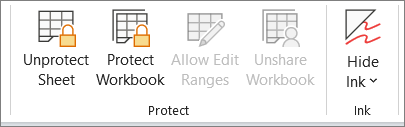
The Protect Sheet option on the ribbon changes to Unprotect Sheet when a sheet is protected. To view this option, select the Review tab on the ribbon, and in Changes, see Unprotect Sheet. Protect Sheet under Review

Unprotect an Excel worksheet

To unprotect a sheet, follow these steps:

Go to the worksheet you want to unprotect.
Go to File > Info > Protect > Unprotect Sheet, or from the Review tab > Changes > Unprotect Sheet.
If the sheet is protected with a password, then enter the password in the Unprotect Sheet dialog box and select OK.

EasetipsNtricks

Insert or delete and Collaborate on Excel