Look up values with VLOOKUP, INDEX, or MATCH
Applies To
Tip: Try using the new XLOOKUP and XMATCH functions, improved versions of the functions described in this article. These new functions work in any direction and return exact matches by default, making them easier and more convenient to use than their predecessors.
Suppose that you have a list of office location numbers, and you need to know which employees are in each office. The spreadsheet is huge, so you might think it is challenging task. It’s actually quite easy to do with a lookup function.
The VLOOKUP and HLOOKUP functions, together with INDEX and MATCH, are some of the most useful functions in Excel.
Note: The Lookup Wizard feature is no longer available in Excel.
Here’s an example of how to use VLOOKUP.
=VLOOKUP(B2,C2:E7,3,TRUE)
In this example, B2 is the first argument—an element of data that the function needs to work. For VLOOKUP, this first argument is the value that you want to find. This argument can be a cell reference, or a fixed value such as “smith” or 21,000. The second argument is the range of cells, C2-:E7, in which to search for the value you want to find. The third argument is the column in that range of cells that contains the value that you seek.
The fourth argument is optional. Enter either TRUE or FALSE. If you enter TRUE, or leave the argument blank, the function returns an approximate match of the value you specify in the first argument. If you enter FALSE, the function will match the value provide by the first argument. In other words, leaving the fourth argument blank—or entering TRUE—gives you more flexibility.
This example shows you how the function works. When you enter a value in cell B2 (the first argument), VLOOKUP searches the cells in the range C2:E7 (2nd argument) and returns the closest approximate match from the third column in the range, column E (3rd argument).

The fourth argument is empty, so the function returns an approximate match. If it didn’t, you’d have to enter one of the values in columns C or D to get a result at all.
When you’re comfortable with VLOOKUP, the HLOOKUP function is equally easy to use. You enter the same arguments, but it searches in rows instead of columns.
Using INDEX and MATCH instead of VLOOKUP
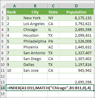
There are certain limitations with using VLOOKUP—the VLOOKUP function can only look up a value from left to right. This means that the column containing the value you look up should always be located to the left of the column containing the return value. Now if your spreadsheet isn’t built this way, then do not use VLOOKUP. Use the combination of INDEX and MATCH functions instead.
This example shows a small list where the value we want to search on, Chicago, isn’t in the leftmost column. So, we can’t use VLOOKUP. Instead, we’ll use the MATCH function to find Chicago in the range B1:B11. It’s found in row 4. Then, INDEX uses that value as the lookup argument, and finds the population for Chicago in the 4th column (column D). The formula used is shown in cell A14.
Give it a try
If you want to experiment with lookup functions before you try them out with your own data, here’s some sample data.
VLOOKUP Example at work
Copy the following data into a blank spreadsheet.
Tip: Before you paste the data into Excel, set the column widths for columns A through C to 250 pixels, and click Wrap Text (Home tab, Alignment group).
| Density | Viscosity | Temperature |
|---|---|---|
| 0.457 | 3.55 | 500 |
| 0.525 | 3.25 | 400 |
| 0.606 | 2.93 | 300 |
| 0.675 | 2.75 | 250 |
| 0.746 | 2.57 | 200 |
| 0.835 | 2.38 | 150 |
| 0.946 | 2.17 | 100 |
| 1.09 | 1.95 | 50 |
| 1.29 | 1.71 | 0 |
| Formula | Description | Result |
| =VLOOKUP(1,A2:C10,2) | Using an approximate match, searches for the value 1 in column A, finds the largest value less than or equal to 1 in column A which is 0.946, and then returns the value from column B in the same row. | 2.17 |
| =VLOOKUP(1,A2:C10,3,TRUE) | Using an approximate match, searches for the value 1 in column A, finds the largest value less than or equal to 1 in column A, which is 0.946, and then returns the value from column C in the same row. | 100 |
| =VLOOKUP(0.7,A2:C10,3,FALSE) | Using an exact match, searches for the value 0.7 in column A. Because there is no exact match in column A, an error is returned. | #N/A |
| =VLOOKUP(0.1,A2:C10,2,TRUE) | Using an approximate match, searches for the value 0.1 in column A. Because 0.1 is less than the smallest value in column A, an error is returned. | #N/A |
| =VLOOKUP(2,A2:C10,2,TRUE) | Using an approximate match, searches for the value 2 in column A, finds the largest value less than or equal to 2 in column A, which is 1.29, and then returns the value from column B in the same row. | 1.71 |
HLOOKUP Example
Copy all the cells in this table and paste it into cell A1 on a blank worksheet in Excel.
Tip: Before you paste the data into Excel, set the column widths for columns A through C to 250 pixels, and click Wrap Text (Home tab, Alignment group).
| Axles | Bearings | Bolts |
|---|---|---|
| 4 | 4 | 9 |
| 5 | 7 | 10 |
| 6 | 8 | 11 |
| Formula | Description | Result |
| =HLOOKUP(“Axles”, A1:C4, 2, TRUE) | Looks up “Axles” in row 1, and returns the value from row 2 that’s in the same column (column A). | 4 |
| =HLOOKUP(“Bearings”, A1:C4, 3, FALSE) | Looks up “Bearings” in row 1, and returns the value from row 3 that’s in the same column (column B). | 7 |
| =HLOOKUP(“B”, A1:C4, 3, TRUE) | Looks up “B” in row 1, and returns the value from row 3 that’s in the same column. Because an exact match for “B” is not found, the largest value in row 1 that is less than “B” is used: “Axles,” in column A. | 5 |
| =HLOOKUP(“Bolts”, A1:C4, 4) | Looks up “Bolts” in row 1, and returns the value from row 4 that’s in the same column (column C). | 11 |
| =HLOOKUP(3, {1,2,3;”a”,”b”,”c”;”d”,”e”,”f”}, 2, TRUE) | Looks up the number 3 in the three-row array constant, and returns the value from row 2 in the same (in this case, third) column. There are three rows of values in the array constant, each row separated by a semicolon (;). Because “c” is found in row 2 and in the same column as 3, “c” is returned. | c |
INDEX and MATCH Examples
This last example employs the INDEX and MATCH functions together to return the earliest invoice number and its corresponding date for each of five cities. Because the date is returned as a number, we use the TEXT function to format it as a date. The INDEX function actually uses the result of the MATCH function as its argument. The combination of the INDEX and MATCH functions are used twice in each formula – first, to return the invoice number, and then to return the date.
Copy all the cells in this table and paste it into cell A1 on a blank worksheet in Excel.
Tip: Before you paste the data into Excel, set the column widths for columns A through D to 250 pixels, and click Wrap Text (Home tab, Alignment group).
| Invoice | City | Invoice Date | Earliest invoice by city, with date |
|---|---|---|---|
| 3115 | Atlanta | 4/7/12 | =”Atlanta = “&INDEX($A$2:$C$33,MATCH(“Atlanta”,$B$2:$B$33,0),1)& “, Invoice date: ” & TEXT(INDEX($A$2:$C$33,MATCH(“Atlanta”,$B$2:$B$33,0),3),”m/d/yy”) |
| 3137 | Atlanta | 4/9/12 | =”Austin = “&INDEX($A$2:$C$33,MATCH(“Austin”,$B$2:$B$33,0),1)& “, Invoice date: ” & TEXT(INDEX($A$2:$C$33,MATCH(“Austin”,$B$2:$B$33,0),3),”m/d/yy”) |
| 3154 | Atlanta | 4/11/12 | =”Dallas = “&INDEX($A$2:$C$33,MATCH(“Dallas”,$B$2:$B$33,0),1)& “, Invoice date: ” & TEXT(INDEX($A$2:$C$33,MATCH(“Dallas”,$B$2:$B$33,0),3),”m/d/yy”) |
| 3191 | Atlanta | 4/21/12 | =”New Orleans = “&INDEX($A$2:$C$33,MATCH(“New Orleans”,$B$2:$B$33,0),1)& “, Invoice date: ” & TEXT(INDEX($A$2:$C$33,MATCH(“New Orleans”,$B$2:$B$33,0),3),”m/d/yy”) |
| 3293 | Atlanta | 4/25/12 | =”Tampa = “&INDEX($A$2:$C$33,MATCH(“Tampa”,$B$2:$B$33,0),1)& “, Invoice date: ” & TEXT(INDEX($A$2:$C$33,MATCH(“Tampa”,$B$2:$B$33,0),3),”m/d/yy”) |
VLOOKUP function
Applies To
Tip: Try using the new XLOOKUP function, an improved version of VLOOKUP that works in any direction and returns exact matches by default, making it easier and more convenient to use than its predecessor.
Use VLOOKUP when you need to find things in a table or a range by row. For example, look up a price of an automotive part by the part number, or find an employee name based on their employee ID.
In its simplest form, the VLOOKUP function says:
=VLOOKUP(What you want to look up, where you want to look for it, the column number in the range containing the value to return, return an Approximate or Exact match – indicated as 1/TRUE, or 0/FALSE).
Paused
Tips:
- The secret to VLOOKUP is to organize your data so that the value you look up (Fruit) is to the left of the return value (Amount) you want to find.
- If you’re a Microsoft Copilot subscriber Copilot can make it even easier to insert and use VLookup or XLookup functions. See Copilot makes lookups in Excel easy.
Technical details
How to get started
There are four pieces of information that you will need in order to build the VLOOKUP syntax:
- The value you want to look up, also called the lookup value.
- The range where the lookup value is located. Remember that the lookup value should always be in the first column in the range for VLOOKUP to work correctly. For example, if your lookup value is in cell C2 then your range should start with C.
- The column number in the range that contains the return value. For example, if you specify B2:D11 as the range, you should count B as the first column, C as the second, and so on.
- Optionally, you can specify TRUE if you want an approximate match or FALSE if you want an exact match of the return value. If you don’t specify anything, the default value will always be TRUE or approximate match.
Now put all of the above together as follows:
=VLOOKUP(lookup value, range containing the lookup value, the column number in the range containing the return value, Approximate match (TRUE) or Exact match (FALSE)).
Examples
Here are a few examples of VLOOKUP:
Example 1
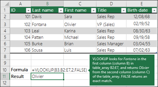
Example 2
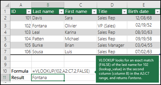
Example 3
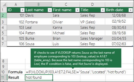
Example 4
Example 5
Common Problems
| Problem | What went wrong |
|---|---|
| Wrong value returned | If range_lookup is TRUE or left out, the first column needs to be sorted alphabetically or numerically. If the first column isn’t sorted, the return value might be something you don’t expect. Either sort the first column, or use FALSE for an exact match. |
| #N/A in cell | If range_lookup is TRUE, then if the value in the lookup_value is smaller than the smallest value in the first column of the table_array, you’ll get the #N/A error value.If range_lookup is FALSE, the #N/A error value indicates that the exact number isn’t found.For more information on resolving #N/A errors in VLOOKUP, see How to correct a #N/A error in the VLOOKUP function. |
| #REF! in cell | If col_index_num is greater than the number of columns in table-array, you’ll get the #REF! error value.For more information on resolving #REF! errors in VLOOKUP, see How to correct a #REF! error. |
| #VALUE! in cell | If the table_array is less than 1, you’ll get the #VALUE! error value.For more information on resolving #VALUE! errors in VLOOKUP, see How to correct a #VALUE! error in the VLOOKUP function. |
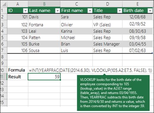
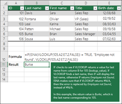
| #NAME? in cell | The #NAME? error value usually means that the formula is missing quotes. To look up a person’s name, make sure you use quotes around the name in the formula. For example, enter the name as “Fontana” in =VLOOKUP(“Fontana”,B2:E7,2,FALSE).For more information, see How to correct a #NAME! error. |
| #SPILL! in cell | This particular #SPILL! error usually means that your formula is relying on implicit intersection for the lookup value, and using an entire column as a reference. For example, =VLOOKUP(A:A,A:C,2,FALSE). You can resolve the issue by anchoring the lookup reference with the @ operator like this: =VLOOKUP(@A:A,A:C,2,FALSE). Alternatively, you can use the traditional VLOOKUP method and refer to a single cell instead of an entire column: =VLOOKUP(A2,A:C,2,FALSE). |
Best practices
| Do this | Why |
|---|---|
| Use absolute references for range_lookup | Using absolute references allows you to fill-down a formula so that it always looks at the same exact lookup range.Learn how to use absolute cell references. |
| Don’t store number or date values as text. | When searching number or date values, be sure the data in the first column of table_array isn’t stored as text values. Otherwise, VLOOKUP might return an incorrect or unexpected value. |
| Sort the first column | Sort the first column of the table_array before using VLOOKUP when range_lookup is TRUE. |
| Use wildcard characters | If range_lookup is FALSE and lookup_value is text, you can use the wildcard characters—the question mark (?) and asterisk (*)—in lookup_value. A question mark matches any single character. An asterisk matches any sequence of characters. If you want to find an actual question mark or asterisk, type a tilde (~) in front of the character.For example, =VLOOKUP(“Fontan?”,B2:E7,2,FALSE) will search for all instances of Fontana with a last letter that could vary. |
| Make sure your data doesn’t contain erroneous characters. | When searching text values in the first column, make sure the data in the first column doesn’t have leading spaces, trailing spaces, inconsistent use of straight ( ‘ or ” ) and curly ( ‘ or “) quotation marks, or nonprinting characters. In these cases, VLOOKUP might return an unexpected value.To get accurate results, try using the CLEAN function or the TRIM function to remove trailing spaces after table values in a cell. |
HLOOKUP function
Applies To
Tip: Try using the new XLOOKUP function, an improved version of HLOOKUP that works in any direction and returns exact matches by default, making it easier and more convenient to use than its predecessor.
This article describes the formula syntax and usage of the HLOOKUP function in Microsoft Excel.
Description
Searches for a value in the top row of a table or an array of values, and then returns a value in the same column from a row you specify in the table or array. Use HLOOKUP when your comparison values are located in a row across the top of a table of data, and you want to look down a specified number of rows. Use VLOOKUP when your comparison values are located in a column to the left of the data you want to find.
The H in HLOOKUP stands for “Horizontal.”
Syntax
HLOOKUP(lookup_value, table_array, row_index_num, [range_lookup])
The HLOOKUP function syntax has the following arguments:
- Lookup_value Required. The value to be found in the first row of the table. Lookup_value can be a value, a reference, or a text string.
- Table_array Required. A table of information in which data is looked up. Use a reference to a range or a range name.
- The values in the first row of table_array can be text, numbers, or logical values.
- If range_lookup is TRUE, the values in the first row of table_array must be placed in ascending order: …-2, -1, 0, 1, 2,… , A-Z, FALSE, TRUE; otherwise, HLOOKUP may not give the correct value. If range_lookup is FALSE, table_array does not need to be sorted.
- Uppercase and lowercase text are equivalent.
- Sort the values in ascending order, left to right. For more information, see Sort data in a range or table.
- Row_index_num Required. The row number in table_array from which the matching value will be returned. A row_index_num of 1 returns the first row value in table_array, a row_index_num of 2 returns the second row value in table_array, and so on. If row_index_num is less than 1, HLOOKUP returns the #VALUE! error value; if row_index_num is greater than the number of rows on table_array, HLOOKUP returns the #REF! error value.
- Range_lookup Optional. A logical value that specifies whether you want HLOOKUP to find an exact match or an approximate match. If TRUE or omitted, an approximate match is returned. In other words, if an exact match is not found, the next largest value that is less than lookup_value is returned. If FALSE, HLOOKUP will find an exact match. If one is not found, the error value #N/A is returned.
Remark
- If HLOOKUP can’t find lookup_value, and range_lookup is TRUE, it uses the largest value that is less than lookup_value.
- If lookup_value is smaller than the smallest value in the first row of table_array, HLOOKUP returns the #N/A error value.
- If range_lookup is FALSE and lookup_value is text, you can use the wildcard characters, question mark (?) and asterisk (*), in lookup_value. A question mark matches any single character; an asterisk matches any sequence of characters. If you want to find an actual question mark or asterisk, type a tilde (~) before the character.
Example
Copy the example data in the following table, and paste it in cell A1 of a new Excel worksheet. For formulas to show results, select them, press F2, and then press Enter. If you need to, you can adjust the column widths to see all the data.
| Axles | Bearings | Bolts |
| 4 | 4 | 9 |
| 5 | 7 | 10 |
| 6 | 8 | 11 |
| Formula | Description | Result |
| =HLOOKUP(“Axles”, A1:C4, 2, TRUE) | Looks up “Axles” in row 1, and returns the value from row 2 that’s in the same column (column A). | 4 |
| =HLOOKUP(“Bearings”, A1:C4, 3, FALSE) | Looks up “Bearings” in row 1, and returns the value from row 3 that’s in the same column (column B). | 7 |
| =HLOOKUP(“B”, A1:C4, 3, TRUE) | Looks up “B” in row 1, and returns the value from row 3 that’s in the same column. Because an exact match for “B” is not found, the largest value in row 1 that is less than “B” is used: “Axles,” in column A. | 5 |
| =HLOOKUP(“Bolts”, A1:C4, 4) | Looks up “Bolts” in row 1, and returns the value from row 4 that’s in the same column (column C). | 11 |
| =HLOOKUP(3, {1,2,3;”a”,”b”,”c”;”d”,”e”,”f”}, 2, TRUE) | Looks up the number 3 in the three-row array constant, and returns the value from row 2 in the same (in this case, third) column. There are three rows of values in the array constant, each row separated by a semicolon (;). Because “c” is found in row 2 and in the same column as 3, “c” is returned. | c |
XLOOKUP function
Applies To
Use the XLOOKUP function to find things in a table or range by row. For example, look up the price of an automotive part by the part number, or find an employee name based on their employee ID. With XLOOKUP, you can look in one column for a search term and return a result from the same row in another column, regardless of which side the return column is on.
Note: XLOOKUP is not available in Excel 2016 and Excel 2019. However, you may come across a situation of using a workbook in Excel 2016 or Excel 2019 with the XLOOKUP function in it, if it was created by someone else using a newer version of Excel.
Paused
Syntax
The XLOOKUP function searches a range or an array, and then returns the item corresponding to the first match it finds. If no match exists, then XLOOKUP can return the closest (approximate) match.
=XLOOKUP(lookup_value, lookup_array, return_array, [if_not_found], [match_mode], [search_mode])
| Argument | Description |
|---|---|
| lookup_valueRequired* | The value to search for *If omitted, XLOOKUP returns blank cells it finds in lookup_array. |
| lookup_arrayRequired | The array or range to search |
| return_arrayRequired | The array or range to return |
| [if_not_found]Optional | Where a valid match is not found, return the [if_not_found] text you supply.If a valid match is not found, and [if_not_found] is missing, #N/A is returned. |
| [match_mode]Optional | Specify the match type:0 – Exact match. If none found, return #N/A. This is the default.-1 – Exact match. If none found, return the next smaller item.1 – Exact match. If none found, return the next larger item.2 – A wildcard match where *, ?, and ~ have special meaning. |
| [search_mode]Optional | Specify the search mode to use:1 – Perform a search starting at the first item. This is the default.-1 – Perform a reverse search starting at the last item.2 – Perform a binary search that relies on lookup_array being sorted in ascending order. If not sorted, invalid results will be returned.-2 – Perform a binary search that relies on lookup_array being sorted in descending order. If not sorted, invalid results will be returned. |
Examples
Example 1 uses XLOOKUP to look up a country name in a range, and then return its telephone country code. It includes the lookup_value (cell F2), lookup_array (range B2:B11), and return_array (range D2:D11) arguments. It doesn’t include the match_mode argument, as XLOOKUP produces an exact match by default.
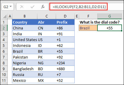
Note: XLOOKUP uses a lookup array and a return array, whereas VLOOKUP uses a single table array followed by a column index number. The equivalent VLOOKUP formula in this case would be: =VLOOKUP(F2,B2:D11,3,FALSE)
———————————————————————————
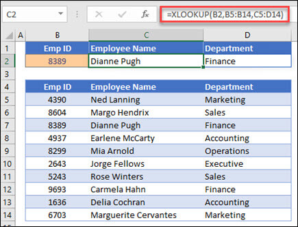
Example 2 looks up employee information based on an employee ID number. Unlike VLOOKUP, XLOOKUP can return an array with multiple items, so a single formula can return both employee name and department from cells C5:D14.
———————————————————————————
Example 3 adds an if_not_found argument to the preceding example.
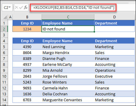
———————————————————————————
Example 4 looks in column C for the personal income entered in cell E2, and finds a matching tax rate in column B. It sets the if_not_found argument to return 0 (zero) if nothing is found. The match_mode argument is set to 1, which means the function will look for an exact match, and if it can’t find one, it returns the next larger item. Finally, the search_mode argument is set to 1, which means the function will search from the first item to the last.
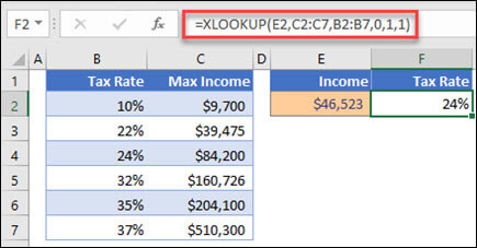
Note: XARRAY’s lookup_array column is to the right of the return_array column, whereas VLOOKUP can only look from left-to-right.
———————————————————————————
Example 5 uses a nested XLOOKUP function to perform both a vertical and horizontal match. It first looks for Gross Profit in column B, then looks for Qtr1 in the top row of the table (range C5:F5), and finally returns the value at the intersection of the two. This is similar to using the INDEX and MATCH functions together.
Tip: You can also use XLOOKUP to replace the HLOOKUP function.
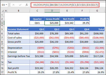
Note: The formula in cells D3:F3 is: =XLOOKUP(D2,$B6:$B17,XLOOKUP($C3,$C5:$G5,$C6:$G17)).
———————————————————————————
Example 6 uses the SUM function, and two nested XLOOKUP functions, to sum all the values between two ranges. In this case, we want to sum the values for grapes, bananas, and include pears, which are between the two.
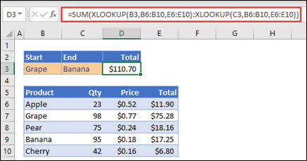
The formula in cell E3 is: =SUM(XLOOKUP(B3,B6:B10,E6:E10):XLOOKUP(C3,B6:B10,E6:E10))
How does it work? XLOOKUP returns a range, so when it calculates, the formula ends up looking like this: =SUM($E$7:$E$9). You can see how this works on your own by selecting a cell with an XLOOKUP formula similar to this one, then select Formulas > Formula Auditing > Evaluate Formula, and then select Evaluate to step through the calculation.
XMATCH function
Applies To
The XMATCH function searches for a specified item in an array or range of cells, and then returns the item’s relative position.
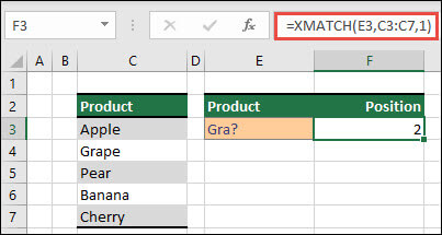
Assume we have a list of products in cells C3 through C7 and we wish to determine where in the list the product from cell E3 is located. Here, we’ll use XMATCH to determine an item’s position within a list.

Syntax
The XMATCH function returns the relative position of an item in an array or range of cells.
=XMATCH(lookup_value, lookup_array, [match_mode], [search_mode])
| Argument | Description |
|---|---|
| lookup_valueRequired | The lookup value |
| lookup_arrayRequired | The array or range to search |
| [match_mode]Optional | Specify the match type:0 – Exact match (default)-1 – Exact match or next smallest item1 – Exact match or next largest item2 – A wildcard match where *, ?, and ~ have special meaning. |
| [search_mode]Optional | Specify the search type:1 – Search first-to-last (default)-1 – Search last-to-first (reverse search).2 – Perform a binary search that relies on lookup_array being sorted in ascending order. If not sorted, invalid results will be returned. -2 – Perform a binary search that relies on lookup_array being sorted in descending order. If not sorted, invalid results will be returned. |
Examples
Example 1
The exact position of the first phrase that exactly matches or comes closest to the value of “Gra” is determined in the example that follow.
Formula: XMATCH(E3,C3:C7,1)
Example 2
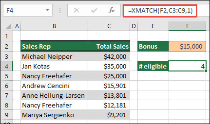
The number of salespeople qualified for a bonus is determined in the following example. In order to discover the closest item in the list or an exact match, this also uses 1 for the match_mode; however, because the data is numeric, it returns a count of values. Since there were four sales representatives that exceeded the bonus amount in this instance, the function yields 4.
Formula=XMATCH(F2,C3:C9,1)
Example 3
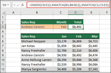
Next, we’ll perform a simultaneous vertical and horizontal lookup using a mix of INDEX/XMATCH/XMATCH. In this instance, we would want the sales total for a certain sales representative and month to be returned. This is comparable to combining INDEX and MATCH methods, but it takes less arguments.
Formula=INDEX(C6:E12,XMATCH(B3,B6:B12),XMATCH(C3,C5:E5))
Example 4
In addition, XMATCH can be used to return a value within an array. =XMATCH(4,{5,4,3,2,1}), for instance, would provide 2 because 4 is the array’s second entry. While =XMATCH(4.5,{5,4,3,2,1},1) produces 1 in this exact match case, the match_mode argument (1) is configured to return either an exact match or the next largest item, which is 5.
