Applies To
The SUM function adds values. You can add individual values, cell references or ranges or a mix of all three.
For example:
- =SUM(A2:A10) Adds the values in cells A2:10.
- =SUM(A2:A10, C2:C10) Adds the values in cells A2:10, as well as cells C2:C10.
Syntax:
SUM(number1,[number2],…)
| Argument name | Description |
|---|---|
| number1 Required | The first number you want to add. The number can be like 4, a cell reference like B6, or a cell range like B2:B8. |
| number2-255 Optional | This is the second number you want to add. You can specify up to 255 numbers in this way. |
Best Practices with SUM
This section will discuss some best practices for working with the SUM function. Much of this can be applied to working with other functions as well.
The =1+2 or =A+B Method – While you can enter =1+2+3 or =A1+B1+C2 and get fully accurate results, these methods are error prone for several reasons:
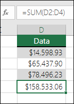
- Typos – Imagine trying to enter more and/or much larger values like this:
- =14598.93+65437.90+78496.23
- #VALUE! errors from referencing text instead of numbersIf you use a formula like:
- =A1+B1+C1 or =A1+A2+A3
Your formula can break if there are any non-numeric (text) values in the referenced cells, which will return a #VALUE! error. SUM will ignore text values and give you the sum of just the numeric values.
- #REF! error from deleting rows or columns
If you delete a row or column, the formula will not update to exclude the deleted row and it will return a #REF! error, where a SUM function will automatically update.
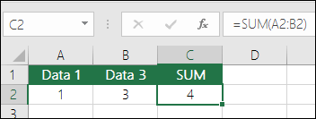
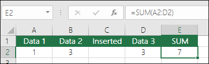
- Formulas won’t update references when inserting rows or columns
If you insert a row or column, the formula will not update to include the added row, where a SUM function will automatically update (as long as you’re not outside of the range referenced in the formula). This is especially important if you expect your formula to update and it doesn’t, as it will leave you with incomplete results that you might not catch.
- SUM with individual Cell References vs. RangesUsing a formula like:
- =SUM(A1,A2,A3,B1,B2,B3)
- =SUM(A1:A3,B1:B3)

Frequently Asked Questions
- I just want to Add/Subtract/Multiply/Divide numbers See Use Excel as your calculator.
- How do I show more/less decimal places? You can change your number format. Select the cell or range in question and use Ctrl+1 to bring up the Format Cells Dialog, then click the Number tab and select the format you want, making sure to indicate the number of decimal places you want.
- How do I add or subtract Times? You can add and subtract times in a few different ways. For example, to get the difference between 8:00 AM – 12:00 PM for payroll purposes you would use: =(“12:00 PM”-“8:00 AM”)*24, taking the end time minus the start time. Note that Excel calculates times as a fraction of a day, so you need to multiply by 24 to get the total hours. In the first example we’re using =((B2-A2)+(D2-C2))*24 to get the sum of hours from start to finish, less a lunch break (8.50 hours total).If you’re simply adding hours and minutes and want to display that way, then you can sum and don’t need to multiply by 24, so in the second example we’re using =SUM(A6:C6) since we just need the total number of hours and minutes for assigned tasks (5:36, or 5 hours, 36 minutes).
For more information, see: Add or subtract time.
- How do I sum just visible cells? Sometimes, when you manually hide rows or use AutoFilter to display only certain data you also only want to sum the visible cells. You can use the SUBTOTAL function. If you’re using a total row in an Excel table, any function you select from the Total drop-down will automatically be entered as a subtotal. See more about how to Total the data in an Excel table.
SUMIF function
Applies To
You use the SUMIF function to sum the values in a range that meet criteria that you specify. For example, suppose that in a column that contains numbers, you want to sum only the values that are larger than 5. You can use the following formula: =SUMIF(B2:B25,”>5″)
Paused
Tips:
- If you want, you can apply the criteria to one range and sum the corresponding values in a different range. For example, the formula =SUMIF(B2:B5, “John”, C2:C5) sums only the values in the range C2:C5, where the corresponding cells in the range B2:B5 equal “John.”
- To sum cells based on multiple criteria, see SUMIFS function.
Important: The SUMIF function returns incorrect results when you use it to match strings longer than 255 characters or to the string #VALUE!.
Syntax
SUMIF(range, criteria, [sum_range])
The SUMIF function syntax has the following arguments:
- range Required. The range of cells that you want evaluated by criteria. Cells in each range must be numbers or names, arrays, or references that contain numbers. Blank and text values are ignored. The selected range may contain dates in standard Excel format (examples below).
- criteria Required. The criteria in the form of a number, expression, a cell reference, text, or a function that defines which cells will be added. Wildcard characters can be included – a question mark (?) to match any single character, an asterisk (*) to match any sequence of characters. If you want to find an actual question mark or asterisk, type a tilde (~) preceding the character.For example, criteria can be expressed as 32, “>32”, B5, “3?”, “apple*”, “*~?”, or TODAY().Important: Any text criteria or any criteria that includes logical or mathematical symbols must be enclosed in double quotation marks (“). If the criteria is numeric, double quotation marks are not required.
- sum_range Optional. The actual cells to add, if you want to add cells other than those specified in the range argument. If the sum_range argument is omitted, Excel adds the cells that are specified in the range argument (the same cells to which the criteria is applied).Sum_range should be the same size and shape as range. If it isn’t, performance may suffer, and the formula will sum a range of cells that starts with the first cell in sum_range but has the same dimensions as range. For example:rangesum_rangeActual summed cellsA1:A5B1:B5B1:B5A1:A5B1:K5B1:B5
Examples
Example 1
Copy the example data in the following table, and paste it in cell A1 of a new Excel worksheet. For formulas to show results, select them, press F2, and then press Enter. If you need to, you can adjust the column widths to see all the data.
| Property Value | Commission | Data |
|---|---|---|
| $100,000 | $7,000 | $250,000 |
| $200,000 | $14,000 | |
| $300,000 | $21,000 | |
| $400,000 | $28,000 | |
| Formula | Description | Result |
| =SUMIF(A2:A5,”>160000″,B2:B5) | Sum of the commissions for property values over $160,000. | $63,000 |
| =SUMIF(A2:A5,”>160000″) | Sum of the property values over $160,000. | $900,000 |
| =SUMIF(A2:A5,300000,B2:B5) | Sum of the commissions for property values equal to $300,000. | $21,000 |
| =SUMIF(A2:A5,”>” & C2,B2:B5) | Sum of the commissions for property values greater than the value in C2. | $49,000 |
Example 2
Copy the example data in the following table, and paste it in cell A1 of a new Excel worksheet. For formulas to show results, select them, press F2, and then press Enter. If you need to, you can adjust the column widths to see all the data.
| Category | Food | Sales |
|---|---|---|
| Vegetables | Tomatoes | $2,300 |
| Vegetables | Celery | $5,500 |
| Fruits | Oranges | $800 |
| Butter | $400 | |
| Vegetables | Carrots | $4,200 |
| Fruits | Apples | $1,200 |
| Formula | Description | Result |
| =SUMIF(A2:A7,”Fruits”,C2:C7) | Sum of the sales of all foods in the “Fruits” category. | $2,000 |
| =SUMIF(A2:A7,”Vegetables”,C2:C7) | Sum of the sales of all foods in the “Vegetables” category. | $12,000 |
| =SUMIF(B2:B7,”*es”,C2:C7) | Sum of the sales of all foods that end in “es” (Tomatoes, Oranges, and Apples). | $4,300 |
| =SUMIF(A2:A7,””,C2:C7) | Sum of the sales of all foods that do not have a category specified. | $400 |
SUMIFS function
Applies To
The SUMIFS function, one of the math and trig functions, adds all of its arguments that meet multiple criteria. For example, you would use SUMIFS to sum the number of retailers in the country who (1) reside in a single zip code and (2) whose profits exceed a specific dollar value.
Paused
Syntax
SUMIFS(sum_range, criteria_range1, criteria1, [criteria_range2, criteria2], …)
- =SUMIFS(A2:A9,B2:B9,”=A*”,C2:C9,”Tom”)
- =SUMIFS(A2:A9,B2:B9,”<>Bananas”,C2:C9,”Tom”)
| Argument name | Description |
|---|---|
| Sum_range (required) | The range of cells to sum. |
| Criteria_range1 (required) | The range that is tested using Criteria1.Criteria_range1 and Criteria1 set up a search pair whereby a range is searched for specific criteria. Once items in the range are found, their corresponding values in Sum_range are added. |
| Criteria1 (required) | The criteria that defines which cells in Criteria_range1 will be added. For example, criteria can be entered as 32, “>32”, B4, “apples”, or “32”. |
| Criteria_range2, criteria2, … (optional) | Additional ranges and their associated criteria. You can enter up to 127 range/criteria pairs. |
Examples
To use these examples in Excel, drag to select the data in the table, right-click the selection, and pick Copy. In a new worksheet, right-click cell A1 and pick Match Destination Formatting under Paste Options.
| Quantity Sold | Product | Salesperson |
|---|---|---|
| 5 | Apples | Tom |
| 4 | Apples | Sarah |
| 15 | Artichokes | Tom |
| 3 | Artichokes | Sarah |
| 22 | Bananas | Tom |
| 12 | Bananas | Sarah |
| 10 | Carrots | Tom |
| 33 | Carrots | Sarah |
| Formula | Description | |
| =SUMIFS(A2:A9, B2:B9, “=A*”, C2:C9, “Tom”) | Adds the number of products that begin with A and were sold by Tom. It uses the wildcard character * in Criteria1, “=A*” to look for matching product names in Criteria_range1 B2:B9, and looks for the name “Tom” in Criteria_range2 C2:C9. It then adds the numbers in Sum_range A2:A9 that meet both conditions. The result is 20. | |
| =SUMIFS(A2:A9, B2:B9, “<>Bananas”, C2:C9, “Tom”) | Adds the number of products that aren’t bananas and are sold by Tom. It excludes bananas by using <> in the Criteria1, “<>Bananas”, and looks for the name “Tom” in Criteria_range2 C2:C9. It then adds the numbers in Sum_range A2:A9 that meet both conditions. The result is 30. |
Common Problems
| Problem | Description |
|---|---|
| 0 (Zero) is shown instead of the expected result. | Make sure Criteria1,2 are in quotation marks if you are testing for text values, like a person’s name. |
| The result is incorrect when Sum_range has TRUE or FALSE values. | TRUE and FALSE values for Sum_range are evaluated differently, which may cause unexpected results when they’re added.Cells in Sum_range that contain TRUE evaluate to 1. Those that contain FALSE evaluate to 0 (zero). |
Best practices
| Do this | Description |
|---|---|
| Use wildcard characters. | Using wildcard characters like the question mark (?) and asterisk (*) in criteria1,2 can help you find matches that are similar but not exact.A question mark matches any single character. An asterisk matches any sequence of characters. If you want to find an actual question mark or asterisk, type a tilde (~) in front of the question mark.For example, =SUMIFS(A2:A9, B2:B9, “=A*”, C2:C9, “To?”) will add all instances with name that begin with “To” and ends with a last letter that could vary. |
| Understand the difference between SUMIF and SUMIFS. | The order of arguments differ between SUMIFS and SUMIF. In particular, the sum_range argument is the first argument in SUMIFS, but it is the third argument in SUMIF. This is a common source of problems using these functions.If you’re copying and editing these similar functions, make sure you put the arguments in the correct order. |
| Use the same number of rows and columns for range arguments. | The Criteria_range argument must contain the same number of rows and columns as the Sum_range argument. |
Sum values based on multiple conditions
Applies To
Let’s say that you need to sum values with more than one condition, such as the sum of product sales in a specific region. This is a good case for using the SUMIFS function in a formula.
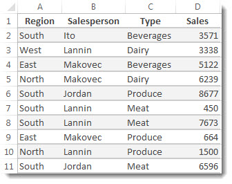
Have a look at this example in which we have two conditions: we want the sum of Meat sales (from column C) in the South region (from column A).
Here’s a formula you can use to acomplish this:
=SUMIFS(D2:D11,A2:A11,”South”,C2:C11,”Meat”)
The result is the value 14,719.
Let’s look more closely at each part of the formula.
=SUMIFS is an arithmetic formula. It calculates numbers, which in this case are in column D. The first step is to specify the location of the numbers:
=SUMIFS(D2:D11,
In other words, you want the formula to sum numbers in that column if they meet the conditions. That cell range is the first argument in this formula—the first piece of data that the function requires as input.
Next, you want to find data that meets two conditions, so you enter your first condition by specifying for the function the location of the data (A2:A11) and also what the condition is—which is “South”. Notice the commas between the separate arguments:
=SUMIFS(D2:D11,A2:A11,”South”,
Quotation marks around “South” specify that this text data.
Finally, you enter the arguments for your second condition – the range of cells (C2:C11) that contains the word “meat,” plus the word itself (surrounded by quotes) so that Excel can match it. End the formula with a closing parenthesis ) and then press Enter. The result, again, is 14,719.
=SUMIFS(D2:D11,A2:A11,”South”,C2:C11,”Meat”)
As you type the SUMIFS function in Excel, if you don’t remember the arguments, help is ready at hand. After you type =SUMIFS(, Formula AutoComplete appears beneath the formula, with the list of arguments in their proper order.
Looking at the image of Formula AutoComplete and the list of arguments, in our example sum_rangeis D2:D11, the column of numbers you want to sum; criteria_range1is A2.A11, the column of data where criteria1 “South” resides.
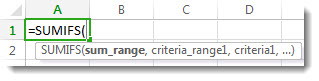
As you type, the rest of the arguments will appear in Formula AutoComplete (not shown here); criteria_range2 is C2:C11, the column of data where criteria2 “Meat” resides.
If you select SUMIFS in Formula AutoComplete, an article opens to give you more help.
Give it a try
If you want to experiment with the SUMIFS function, here’s some sample data and a formula that uses the function.
You can work with sample data and formulas right here, in this Excel for the web workbook. Change values and formulas, or add your own values and formulas and watch the results change, live.
Copy all the cells in the table below, and paste into cell A1 in a new worksheet in Excel. You may want to adjust column widths to see the formulas better
| Region | Salesperson | Type | Sales |
|---|---|---|---|
| South | Ito | Beverages | 3571 |
| West | Lannin | Dairy | 3338 |
| East | Makovec | Beverages | 5122 |
| North | Makovec | Dairy | 6239 |
| South | Jordan | Produce | 8677 |
| South | Lannin | Meat | 450 |
| South | Lannin | Meat | 7673 |
| East | Makovec | Produce | 664 |
| North | Lannin | Produce | 1500 |
| South | Jordan | Meat | 6596 |
| Formula | Description | Result | |
| =SUMIFS(D2:D11,A2:A11,”South”, C2:C11,”Meat”) | Sums the Meat Sales in Column C in the South region in Column A | 14719 |
